Turbulence-degraded wave fronts as fractal surfaces - Physics ...

444 J. Opt. Soc. Am. A/Vol. 11, No. 1/January 1994 

Turbulence-degraded wave fronts as fractal surfaces 

C. Schwartz, G. Baum, and E. N. Ribak 

Department of Physics, Technion-Israel Institute of Technology, Technion City, Haifa 32000, Israel 

Received January 7, 1993; revised manuscript received April 29, 1993; accepted June 8, 1993 

We identify wave fronts that have passed through atmospheric turbulence as fractal surfaces from the Fractional 

Brownian motion family. The fractal character can be ascribed to both the spatial and the temporal behavior. 

The simulation of such wave fronts can be performed with fractal algorithms such as the Successive Random 

Additions algorithm. An important benefit is that wave fronts can be predicted on the basis of their past measurements. 

A simple temporal prediction reduces by 34% the residual error that is not corrected by adaptiveoptics 

systems. Alternatively, it permits a 23% reduction in the measurement bandwidth. Spatiotemporal 

prediction that uses neighboring points and the effective wind speed is even more beneficial. 

1. INTRODUCTION 

We examine the phase of light that has passed through 

a turbulent atmosphere. The degraded wave front is a 

homogeneous and isotropic stochastic Gaussian process.' 

This process is well described by a structure function that 

behaves like a power law over many scales of length in 

the so-called inertial range. This range lies between the 

inner scale, which is of the order of a few millimeters, and 

the outer scale, which is of the order of the height above 

the ground. This structure function can be written as' 

r 5/3 

Dq,(r) = ([p(R + r) - p(R)] 2 ) = 6 . 8 8 (f) (1) 

\ro/ 

where r is the well-known Fried length. We obtain this 

expression analytically by using the Kolmogorov assumptions 

concerning the power spectrum of velocity and temperature 

fluctuations in a turbulent medium. The 

validity of this function (at least for the case of astronomical 

imaging) has been demonstrated in many observations. 

2 From dimensional reasoning it is evident that the 

power spectrum of the wave-front phase also has a powerlaw 

dependence (which we call the Kolmogorov power spectrum) 

on the spatial frequency K: 

P,(K) xc . (2) 

2. FRACTIONAL-BROWNIAN-MOTION 

SURFACES 

The relations that are given above resemble a mathematical 

entity called Fractional Brownian motion (FBm). 3 ' 4 A 

Brownian process B(t) (e.g., in one dimension, the temporal 

one) is a Gaussian stochastic process characterized by 

an incremental variance that is proportional to time: 

([B(T + t) - B(T)] 2 ) t. (3) 

An extension is the FBm, Bh, for which 

([Bh(T + t) - Bh(T)] 2 ) C t2H, (4) 

where H is the Hurst parameter 4 and is in the range 0-1. 

For extension to higher dimensions one changes the 

0740-3232/94/010444-08$06.00 © 1994 Optical Society of America 

Schwartz et al. 

scalars to vectors, and the variance is proportional to the 

vector modulus. For H = 0.5 the process is a classical 

Brownian motion [relation (3)]. Again using dimensional 

analysis, we find that the power spectrum of the FBm 

was 3 - 5 

PB(K) cc-(2H+E) (5) 

where E is the standard topological dimension of the generalized 

surface. Thus, for a curve, E = 1; for a surface 

(such as a wave front), E = 2, etc. This kind of stochastic 

process is found to describe many natural phenomena 

such as the discharge of rivers, the Earth's relief, clouds, 

and 1/f noise. The generalized surface is a fractal in a 

self-affine way, i.e., the surface is statistically similar for 

all scale lengths, but the dependent variable (in this case, 

the phase) is scaled differently from the space dimensions. 4 

A characterizing parameter of fractals is their dimension 

(also called the Hausdorff dimension), which is always 

greater than the topological dimension E. The difference 

between the two describes the ruggedness of the surface. 

Thus a highly convoluted and complex line will almost fill 

a two-dimensional plane, whereas a slightly crinkled paper 

will remain almost two dimensional. The fractal 

3 5 

dimension of the FBm surface was found to be 

F = E+ 1 - H. (6) 

Thus we identify the wave front (within the inertial range) 

as a FBm with a Hurst parameter H = 5/6 and a fractal 

dimension F = 13/6. The fractal nature of turbulencerelated 

phenomena was first established by Mandelbrot, 3 

who dealt with the fractal dimension of isothermal surfaces 

in a turbulent medium. To our knowledge, we are 

the first to identify wave fronts passing through a turbulent 

atmosphere as fractal surfaces. Fractal properties 

can also be related directly to the time behavior if one 

assumes the Taylor or frozen-flow description of the atmosphere. 

2 The turbulent eddies are driven by a constant, 

uniform wind across the optical aperture in a velocity v 

that does not permit a significant development during the 

transit time _ ro/v. Crosswinds at different layers 

change the time to r _ r/Av, where Av is related to the 

velocity dispersion. 2 Modern telescopes have a single


.) 

a) 

CJ 

In 

0 

1000 

100 

10 

1 10 100 

Frequency 

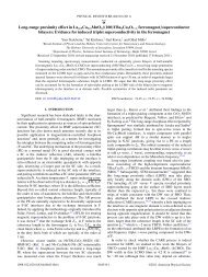
Fig. 1. Power spectrum of a one-dimensional FBm generated by 

the SRA algorithm (averaged over 2000 realizations) compared 

with the expected 8/3 power law. High frequencies are noisy because 

of numerical errors. 

dominant layer, so the velocity dispersion is rather small, 

and the frozen-flow description is usually valid. 

The time behavior of a point on the wave-front surface 

is the trace that is obtained when this surface is cut by a 

plane that is perpendicular to it in the direction of the 

wind. Since this trace is a one-dimensional curve, the 

fractal dimension is now 13/6 - 1 = 7/6. We deduce that 

the Hurst parameter is again 5/6 and that the power-law 

exponent of the temporal power spectrum is -8/3, as is 

well known. 6 The character of the temporal (and the spatial) 

power spectrum does not change when there are 

several cascaded turbulent layers, but it cannot be related 

so simply to the wind velocity. 

The correlation function of a FBm process is, according 

to the Wiener-Khinchine theorem, the Fourier transform 

of the power spectrum. Unfortunately it is not defined, 

since the Fourier transform does not converge for the 

range of exponents in question. We deal with this point 

in Section 4 and in Appendix A. 

What can we gain from the identification of the wave 

front as a fractal surface? We present two implications: 

simulation and prediction. 

3. SIMULATION 

~~~~~~~~............. ......... ..... . .. , -,- 

......................................................- - - i - ; s - 

. ............. .. .. ................... . . . .. 

~. .. .. . . . . ... .. . .. . . . ... . .... . . .. . . . 

........................... ............................................... ................................. I 

. . . . . . . . . . . .. . . . . . . . . , .. . . . . . . . . ... . . . 

.. . . .. . . 

.......... 

...... . .. . .. . .. . 

~~~~~~~~~~............ 

. .................. ........ .......... ! 

. . . . . .............. .. ........ . ........ ... ... 

.~ ~ .. .. .. . . .. .. .. . . . . . .. ....... 

~~~~~~~.............. 

' AL , .......... 

1 -.............................................. :: ::::'::: :::::: 

............................................... ................I 

.......................... ,.,.,.;.,.,.,.I 

.. . ............ .... --- , .............. 

... .. .. ... .. .. .. .. .. . . .. . . .... .... .. 

The need for simulations of turbulence-degraded wave 

fronts has arisen in some areas. The first was for exploration 

of new algorithms for phase retrieval. Later 

it became necessary to simulate the performance of 

adaptive-optics systems or other optical instruments and 

data-processing algorithms. Many algorithms`~ have 

been suggested for this purpose, and most of them are 

based on some type of spectral synthesis, which requires 

one or two Fourier-transform stages. Each transform 

requires approximately N log N computer operations, 

where N is the number of points in the array. Since we 

have identified the degraded wave front as a fractal surface, 

we can benefit from the wealth of algorithms suggested 

for generating fractal surfaces. 

Vol. 11, No. 1/January 1994/J. Opt. Soc. Am. A 445 

An algorithm that was suggested for efficient fractal 

construction is the Successive Random Additions (SRA) 

algorithm. It can be used to produce one-dimensional 

traces (temporal behavior) and surfaces (wave fronts) and 

is based on building a finer and finer grid with the required 

correlation function. 5 The number of operations 

to create the same array of N points is now of the order of 

N rather than N log N. Figure 1 is a comparison between 

the known power law and an average power spectrum 

that we obtained by using SRA algorithm for the 

temporal case. We can deduce that the algorithm will 

yield a good coarse simulation, but where small scale (high 

frequency) is important the realizations are too noisy because 

of numerical errors in the computer. When only 

low-order aberrations are important, this algorithm is a 

fast and simple generator of wave-front realizations. 

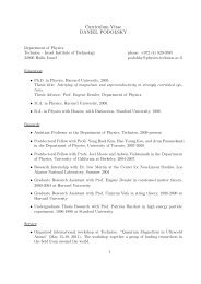
Figure 2 presents one realization of a wave front and the 

speckle pattern that was obtained through the aperture as 

depicted for a monochromatic point source. 

4. PREDICTION 

The Hurst parameter that is related to the turbulencedegraded 

wave front is 5/6. This value implies a persistent 

character in both the spatial and the temporal domains. 

This persistence can be demonstrated if we 

calculate a normalized correlation measure of past and 

future increments (where we define the present as zero) 3 : 

(-Bh(-t)Bh(t)_ 1 ([Bh(t) - Bh(-t)] 2 ) - 2([Bh(t)]) 

([Bh(t)1 ) 2 [Bh(t)] ) 

'/2 (2t)2H - t2H 

t2H 

= 2 2H-1 - 1. (7) 

For H = 0.5 the process is completely uncorrelated; for 

H < 0.5 the process is antipersistent; for H > 0.5 the 

process is persistent, having a positive correlation between 

past and future without dependence on time. This implies 

that we can use predictive algorithms to decrease 

the error that is induced by control time lag in adaptiveoptics 

systems.1 0 Below we present an approach that is 

different from former studies that have assumed a chaoticattractor" 

behavior. This is not necessarily contradictory, 

since fractal dimensions are related to chaotic 

processes. Statistical prediction for adaptive optics has 

been explored earlier, but not in this manner.' 2 

The simplest predictor is a linear estimator,' 3 in which a 

future phase at some point is estimated by a linear combination 

of past phase measurements. We assume that the 

phase p(x, y, t) is measured on a spatial grid of Ax = Ay = 

1, which is small compared with the aperture and the 

outer scale, and in time steps At, which are small compared 

with the coherence time of the atmosphere. The 

general structure of the estimator of the phase in a grid 

point (x, y) is 

(x, y, t) = I rixk(x + iAx, y + jAy,t - kAt). 

ijk 

Now we consider the temporal case alone, where 

(8)


0 50 100 1 50 200 250 

(a) 

l 

IMAGE 

100 150 

Fig. 2. (a) Realization of a wave front generated by the SRA algorithm. 

(b) The speckle pattern of a monochromatic point 

source through the aperture and the wave front shown in (a). 

N 

WAVE FRONT 

0(t = E ri(p(t - iAt). 

i 

The mean-square error (MSE) is defined as 

IN 

(e2) = ((P(t) - 0(t)12 K ) = (t) - rip(t - iAt) 2) 

N N 

= F(0) + Er,2r(o) - 2rjr(iAt) 

i i 

N 

+ 2ZrirjrF(Ii - jAt), 

i>j 

(9) 

where 

(11) 

is the temporal correlation function between consecutive 

wave-front phases. We now use the identity 

1 2 (12) 

Note that CT 2 H is the structure function [Eq. (1)]. After 

some algebra we can write 

N 2 

(,62) =]F(O) ri 

N N 

+ 7-ri (iAt)2Hf _Erirj(i - jAt) 2H 

i i>j 

(13) 

Since F(0) is infinite for an ideal FBm, we need to obtain a 

finite value for the error. To this end we impose the 

normalization constraint 

N 

Er = 1. 

i 

(14) 

Minimizing with respect to each r under the above 

constraint, we obtain a set of linear equations that can be 

solved for any length of estimator that is required. The 

set of coefficients and the MSE for a few cases (for H = 

5/6) are presented in Table 1. 

We can see immediately that the improvement over 

using the simplest predictor is insignificant. The coefficients 

are different from those of the simple extrapolation 

case, which for N = 2 are ri = {2, -1}. 

To introduce a finite outer scale we retrace our steps 

and again write the entire phase estimator as 

O(x, y, t) = rjkp(x + iAx, y + jAy, t - kAt) R , 

ijk 

(15) 

where R is the vector of the estimator coefficients and 1D 

is a vector containing past measurements on grid points 

(i, j, k). Our goal is to minimize the MSE 

(E2) = ([sp(x, y, t) (x, y, t)] 2) 

= ([(p(x, y, t) - RTqD] 2) = (2) - 2RT(q4) + RT(IDDT)R 

Table 1. Sets of Coefficients and Mean-Square 

Errors for Four Linear-Predictor Lengths 

Mean-Square 

N Coefficients (re) Error ((e 2 )) 

la {1} 

51 3 

cAt 

2b {1.58740,-0.58740} 0.654960cAt 13 

3 {1.47946, -0.344348, -0.153114} 0.639605cAt 5 / 3 

4 {1.47942, -0.384921,0.0233227, -0.117827} 

5 /3 

0.630725cAt 

(10) 'Simple time lag. 

bTwo-point temporal prediction. 

r(T) = (0(00t - T)) 


( 2 - 2RTP + RTMR. (16)


We obtain the minimizing set of estimator coefficients by 

performing a gradient in R space and equating it with 

zero. The result is 

Rm = M-1P 

The value of the minimum squared error obtained is 

(E 2 )m = (p2) _ pTR. 

(17) 

(18) 

The presence of uncorrelated noise will not change Rm but 

will increase the error by the amount of power that is contained 

in the noise. 

We now apply this theory of linear predictors to the case 

of adaptive optics. This calls for the calculation of spatiotemporal 

correlation terms in the matrix M and the vector 

P of the general form 

(@p(x + iAx,y + jy,t - kAt)qp(x,y,t)). (19) 

It is possible to measure these terms directly (e.g., interferometrically 

2 ). However, we can find a simple solution 

by using the frozen-flow assumption, whereby these terms 

can be transformed to 

(So(x + iAx + kvxAt, y + jy + kvyAt, t)s(x, y, t)) r(r). 

(20) 

Here v and v are the components of the wind speed v, 

and 

r = [(iAx + kv.At) 2 + (jAy + kv At) 2 ]" 2 . (21) 

The correlation function is the Fourier transform of the 

power spectrum. However, the correlation function of a 

FBm is not defined because the transform of the power 

spectrum in relation (5) does not converge, and we must 

employ one of several modifications. One possible modification 

is to assume a constant power from zero up to a 

certain low frequency (Ko) corresponding to the outer scale 

of the turbulence, and from this point a decrease according 

to the -11/3 power law [relation (2)]. This modification 

is not considered here since it gives too much weight 

to very low spatial frequencies corresponding to length 

scales that are much larger than the outer scale. Another 

possibility is to ignore any contribution from the frequencies 

that are lower than Ko (having a cut-on at Ks). Another 

common way is to add a constant in quadrature to 

the spatial frequency to yield a form that is similar to the 

von Kdrmdn power spectrum (we ignore the small modification 

at high frequencies): 

P c(K) x (K 2 + K0 2 )11/6. (22) 

We can use both these modifications to calculate the correlation 

terms and especially the normalized correlation 

y(r) F(r)/F(0). From Appendix A we obtain for the cuton 

modification 

y(r) 1 - 1.864(Kor)5 13 + 1.25(Kor) 2 + O(Kor)"1/ 3 

and for the von Karman modification 

(23) 

y(r) - 1 - 1.864(Kor)5/3 + 1.5(Kor) 2 + O(Kor)"1/ 

3 . (24) 

Up to the first significant term the approximations are 

the same. Below we neglect the second-order term, even 


though in the worst case Kor is _10-2 (c 0 0.1 m- 3 , r 

0.1 m), and this term is smaller than the first-order term 

only by a factor of 5. For more favorable cases the situation 

is much improved. Two examples are as follows: 

(1) Let us examine a two-point estimator of the form 

(x,y,t) = rp(x,y,t - At) + r2 (P(X,y,t - 2At), (25) 

i.e., we try to predict the wave front by using two former 

measurements in the same place. The normalized matrix 

M and vector P are 

M = - Ght 5 13 1 ] ' 

[p - GAt 3 13 1 

1 - G(2t)513 

(26) 

(27) 

where G is a function of the cut-on frequency Ko and the 

wind speed v: 

G = 1.864(Kov) 5 13 . (28) 

After performing matrix inversion and using Eq. (10), we 

choose to retain the independent terms in the solution and 

obtain 

[ 22/31 1.587401 

(29) 

m - 1 - 22/3J [-0.58740] 

These coefficients are the same as those that were obtained 

for the case of the ideal FBm. See Fig. 3 for the 

results of a numerical simulation. 

Using more points in At results in a more complex but 

also more accurate estimator for the cases in which outerscale 

considerations are important. If the exact value of 

the parameters is not known, then we can use a search 

algorithm and can optimize on some measure of the image 

quality, or we can use a neural network.' 4 We need to 

remember that, regardless of how many coefficients we 

0.95 

o0.85 

0.7 

0.65 

1 

1.1 1.2 1.3 1.4 1.5 1.6 1.7 1.8 1.9 

Extrapolation parameter 

Fig. 3. Numerical simulation of two-point temporal extrapolation. 

The MSE is plotted versus the first extrapolation parameter, 

and it is normalized to unity in the simple-lag case.

448 J. Opt. Soc. Am. A/Vol. 11, No. /January 1994 

( a ) 

t = At 

=0 

t = At 

= 0 

= -At 

( b ) 

Fig. 4. Two spatiotemporal prediction schemes: (a) with nine 

points in one past layer and (b) with six points in two past layers. 

use or how many orders we consider, the only parame 

are Ke, v,, vy. 

(2) In a more complex example we try to use meassure 

ments that were made in the previous time intervwal 

at 

and around the point of interest. The grid points tha.t 

we 

use are 

x - Ax,y - Ay x,y - Ay x + Ax,y - Ay 

x - Ax,y x,y x + Ax,y 

x - Ax,y + Ay x,y + Ay + Ax,y + Ay 

eters 

The vector P is a function of spatiotemporal coordinates, 

and the squared distances that are required for the 

computations of the correlation terms are 

(AX - vAt) 2 + (Ay - VyAt) 2 

(v.At) 2 + (Ay - v At) 2 

(Ax + VAt) 2 + (Ay - VyAt) 2 

(Ax - hAt) 2 + (At) 2 

(VXAt) 2 2 

+ (At) 

(AX + vAt) 2 + (VyAt) 2 

(AX - VXAt) 2 + (Ay + VyAt) 2 

(v"At) 2 + (Ay + v t) 2 

(Ax + vAt) 2 + (Ay + VyAt) 2 

* (32) 

The resulting estimator kernel, up to the first order in 

At, is 

0.004(vX + O)At/l 0.518vyAt/l 0.00 4 (-v, + vy)At/l 

0.518vAt/l 1 -0.518vAt/l . 

0.004(v, - v)At/l -0.518vyAt/l -0.004(v, + v,)At/l 

(33) 

This kernel, as in example (1), complies with the required 

condition that the sum of coefficients be unity for the solution 

not to blow up with time. There is no dependence 

on Ko in this order. If we assume a wind in the x direction, 

then the kernel is approximated by 

0.004vAt/l 

0.518v.At/l 

0.004v.,At/l 

0 -0.004vxAt/l 

1 -0.518vxAt/l 

0 -0.004v.At/l 


(34) 

The result that is obtained from a direct one-dimensional 

derivation is the estimator kernel 

[0.525vxAt/ 1 -0.525vxAt/l]. (35) 

If we regard this kind of prediction as a trivial interpo- 

(30) lation on the sampled signal, we obtain a result that is 

rather similar to expression (35): 

[see also Fig. 4(a)]. All the measurements are from time [0.5vxAt/ 1 -0.5vxAt/l]. (36) 

t - At. The M matrix is now a 9 9 matrix. The order 

of the coefficients is from the upper left-hand corner g oing 

toward the right and downward. Here we use the assumption 

that both the x and they intervals are equal to 1. 

The terms of the matrix depend only on spatial co( )rdinates 

since we use information from the same time iriter- 

val. To simplify the presentation we show the matri.x 

of 

distances for the computation of the correlation termis 

in 

units of 1: 

The MSE's for expressions (35) and (36) are quite similar, 

but expression (35) does indeed give the smaller one. 

These results were also verified by a one-dimensional 

numerical simulation. 

Another predictor that we considered utilizes informa- 

tion that is obtained in six samples: the point for which 

we seek to predict and its four nearest neighbors (with the 

data for all five being collected in the previous sample 

time), and the same grid point two time intervals ago [see 

0 

1 

1 

0 

2 

1 

1 

V2 1 

2 

2 V 

Fig. 4(b)]. Until now we have considered only the first 

order in the predictor expansion. In Figs. 5 and 6 we present 

the results of the full numerical treatment for the 

2 1 

1 V5_ 2 

MSE surfaces. It is clear that much better results can be 

1 

1 2 1 

obtained with a spatiotemporal prediction than with a 

2 

V5 

1 

2 

1 2 

V 1 

v vl 

2 V 

02 

1 

1 

1 

0 

1 

0 

1 

2 

1 V2 

V 1 

1 2 

0 1 

1 0 

(31) temporal prediction. The drawback is that knowledge of 

the wind's effective speed and direction is required. 

We assumed that the phase signal was sampled discretely. 

Usually the phase sensor does sample the wave 

front, but the imager integrates over time, so the phase 

error must be minimized over the entire sample period



and not just at the sample points. In Appendix B we examine 

modifications that arise from this integration. 

Any improvement that is obtained from applying prediction 

algorithms is dependent on the control scheme that is 

used. In Appendix B we show that the residual error decreases 

by a factor of 1.5 because of temporal prediction. 

Alternatively, if we set a temporal rms residual error of 0.1 

wavelength as our goal, we learn, using a calculation similar 

to that of Appendix B, that the sample rate for a nonpredictive 

mode is 

(a) (37) 

\ro / 

° * 5- _V-l 

(c) 

Fig. 5. MSE for three cases: (a) simple lag (no prediction), 

equal to the structure function, with the structure constant being 

taken as unity; (b) spatiotemporal nine-point prediction 

[Fig. 4(a)]; 

SO 

9us 

(c) spatiotemporal 

.. 

six-point 

,. 

prediction 

2 

[Fig. 4(b)]. 

x and y units are vAr/l. 

1. 

1 .2no 

prediction 

wj 0. 

2! 

0. 

0. 

(b) 

where ve is an effective wind speed defined by 

(38) 

For the two-point predictor we have an improved sample 

rate of 

points 

APPENDIX A 

6 points 

points 

0 0.2 0.4 0.6 0.8 1 1.2 1.4 1.6 1.6 2 

Displacement 

Fig. 6. Cartesian cuts through the MSE surfaces (see Fig. 5) for 

simple lag, two-point prediction, six-point prediction, and ninepoint 

prediction. Displacement units are again vAT/l, and the 

MSE is scaled by the structure constant. 

\ro/ 

(39) 

We have yet to determine the optimal estimator. We 

showed above that temporal prediction with more than two 

samples results in only a marginal improvement but that 

use of a spatiotemporal-prediction scheme will reduce the 

bandwidth requirements even further. The exact values 

of this bandwidth are yet to be calculated. 

5. CONCLUSIONS 

We have described the fractal character of turbulencedegraded 

wave fronts. Algorithms for the generation of 

fractal surfaces can be used in simulating wave fronts. 

Correlations embedded in the wave-front surface can be 

employed to explain the validity of using prediction algorithms. 

We have examined simple statistical prediction 

schemes. The MSE can be reduced, or, alternatively, the 

spatial- and temporal-bandwidth requirements of the 

adaptive-optics system can be relaxed. 

We examine two possible ways of modifying the theoretical 

power spectrum of the phase fluctuations to calculate the 

normalized correlation terms that are required for our 

computations. The first is to make a cut-on at the spatial 

frequency that is related to the outer scale. The second is 

to use the von Kdrmdn modification. The two modifications 

are summarized as follows: 

p (co)(K) = ClK -11/3 K 2 KO, 

p(VI (K) = C 2(K 2 + Ko 2 )11/3, K 2 0. 

(Al) 

(A2) 

To obtain the correlation function we perform the 

Fourier transform of the power spectrum. After the 

angular integration we obtain, for both choices,


(a) 

sampling points 

(b) 

time 

time 

Fig. 7. Adaptive-mirror control schemes. (a) The mirror is held 

at the last sampled value until the wave front is sampled again. 

(b) The mirror is moved linearly to a predicted value. No lag is 

assumed in both cases, and the mirror is moved instantly to the 

next sampled point. 

F(r) = 2 f d,,P,(K) Jo(Kr). 

For the cut-on case we obtain 

1/ 5 0 r 

F,(r) = 2Cl() 0.6k F2 - 6o ( - - 

- 1.11833(Kor)5/3}, 

(A3) 

(A4) 

where F 2 is a generalized hypergeometric function. If 

we use the first terms in the series expansion, we have 

F,(r) 2TC,[0.6K 

5 /3 - 1.11833r5 13 

+ 0.75K,&"/ 

3 r 2 + 0(r)"11 3 ]. (A5) 

The normalized correlation function is defined as y(r) = 

F(r)/F(0), or, for the cut-on case, 

y,(r) 1 - 1.863890r)5/ 3 + 1.25(i 0 r) 2 + (r) " 3 . (A6) 

After the spatial integration we obtain, for the 

von Karman case, 

F 2 (r) = 2rC 20.59664KO-5/6r 6 K 5 1 6 (Ko r), 

(A7) 

where K is a modified Bessel function of the second kind. 

The first terms in the expansion are 

F 2(r) 2C 2[0.6Ko` 5 3 - 1.11833r5 3 

+ 0. 9 KO-; Vr 2 + 0(r)1/3], 

and the normalized correlation is 

y 2 (r) 1 - 1.86389(Kor) 

I mirror wave front 

I I 

- o 

(A8) 

1 3 + 1.5(Kor) 2 + 0(r)"11 3 . (A9) 

The constants Cl, C2 in the expressions for the power 

spectra [Eqs. (Al) and (A2)] are deduced from the requirement 

that the correct form of the structure function, 

D,(r) = 6.88(r/ro) 1 3 [Eq. (1)], is to be maintained. For example, 

for the von Kdrmdn case 

APPENDIX B 

C 2 = 0.4896ro 51 3 . (A10) 

In the text of this paper we attempt to minimize the error 

in a discretely sampled signal. The wave-front sensor 

does sample the phase in intervals, but the imager integrates 

over it. Let us assume that the deformable mirror, 

which acts as the wave-front-correction device, responds 

instantly and that we are limited only by the sampling 

rate. If we do not use any prediction, then the mirror is 

held after the sample [Fig. 7(a)], and the MSE over the 

sample period is 

1 A t =5/3 A t 3 

(,e 2 ) = -J 6.88 dt = 0.375 6.88 

(Bi) 

Let us now assume that we use a linear estimator to predict 

the next point, move the mirror linearly to that point, 

and then immediately correct to the new sampled point 

[Fig. 7(b)]. The MSE will be 

(E ') o (°p(t) -{p(O) + [rp(0) 

-()+ 

+ (1 - r)p(-At)]) dt)- (B2) 

After some integrations we obtain 

62) A t 51 ) 

(e 2 ) = 6.88 -) [0.375 + 0.333(1 - r) 2 + 0.412(1 - r)]. 

(B3) 

Minimizing with respect to r, we find that r = 1.618, 

which is slightly different from what we found in Eq. (29). 

The value at the minimum is (e 2 ) = 0.248 5 3 

X 6.88(At/To) , 

which is significantly smaller than Eq. (Bi). Using the 

estimator from Eq. (29) does not result in a noticeable 

increase. 

ACKNOWLEDGMENTS 

The authors thank S. G. Lipson for his helpful comments. 

This research was supported in part by the Ministry of 

Science and Technology. Additional support was available 

from the Jet Propulsion Laboratory, California Institute 

of Technology. 

REFERENCES 


1. J. W Goodman, Statistical Optics (Wiley-Interscience, 

New York, 1985). 

2. F. Roddier, "The effects of atmospheric turbulence in optical 

astronomy," in Progress in Optics XIX, E, Wolf, ed. (North- 

Holland, Amsterdam, 1981), Chap. V, p. 307. 

3. B. B. Mandelbrot, Fractals. Forms, Chance and Dimension 

(Freeman, San Francisco, Calif., 1977). 

4. R. F. Voss, "Random fractals: self-affinity in noise, music, 

mountains and clouds," Physica D 38, 362-371 (1989).


5. H. 0. Peitgen and D. Saupe, eds., The Science of Fractal 

Images (Springer-Verlag, Berlin, 1987), Chap. 2, pp. 71-136. 

6. S. F Clifford, "Temporal frequency spectra for a spherical 

wave propagating through atmospheric turbulence," J. Opt. 

Soc. Am. 61, 1285-1292 (1971). 

7. E. Ribak, "Phase relations and imaging in pupil plane interferometry," 

in NOAO-ESO Conference on High-Resolution 

Imaging by Interferometry, F Merkle, ed., Vol. 29 of European 

Southern Observatory Conference and Workshop Proceedings 

(European Southern Observatory, Garching, 

Germany, 1988), pp. 271-280. 

8. R. Barakat and J. W Beletic, "Influence of atmospherically 

induced random wave fronts on diffraction imagery: a computer 

simulation model for testing image reconstruction 

algorithms," J. Opt. Soc. Am. A 7, 653-671 (1990). 


9. G. Welsh and R. Phillips, "Simulation of enhanced backscatter 

by a phase screen," J. Opt. Soc. Am. A 7, 578-584 (1990). 

10. T. J. Kane, C. S. Gardner, and L. A. Thompson, "Effects of 

wave front sampling speed on the performance of adaptive 

astronomical telescopes," Appl. Opt. 30, 214-221 (1991). 

11. M. B. Jorgensen, G. J. M. Aitken, and E. K. Hege, "Evidence 

of a chaotic attractor in star-wander data," Opt. Lett. 16, 64- 

66 (1991). 

12. V E. Zuev and V P. Lukin, "Dynamic characteristics of optical 

adaptive systems," Appl. Opt. 26, 139-144 (1987). 

13. B. Widrow and S. D. Steams, Adaptive Signal Processing 

(Prentice-Hall, Englewood Cliffs, N.J., 1985). 

14. M. B. Jorgensen and G. J. M. Aitken, "Prediction of atmospherically 

induced wave-front degradations," Opt. Lett. 17, 

466-468 (1992).

Turbulence-degraded wave fronts as fractal surfaces - Physics ...

Create successful ePaper yourself

Delete template?

Save as template?