Dual fronts in a phase field model
Dual fronts in a phase field model
Dual fronts in a phase field model

You also want an ePaper? Increase the reach of your titles
YUMPU automatically turns print PDFs into web optimized ePapers that Google loves.
Abstract<br />
Physica D 146 (2000) 328–340<br />
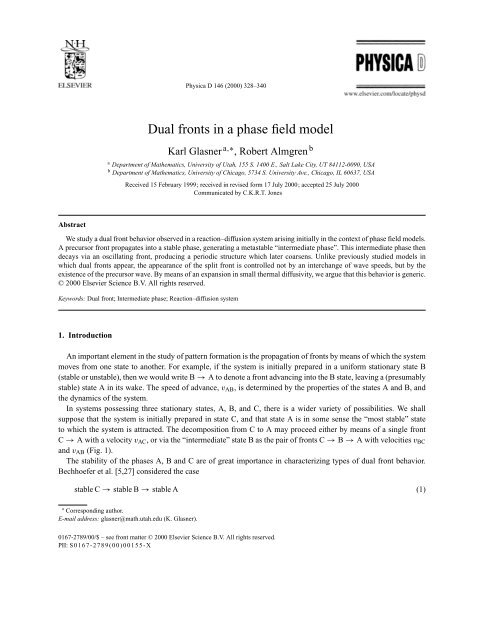
<strong>Dual</strong> <strong>fronts</strong> <strong>in</strong> a <strong>phase</strong> <strong>field</strong> <strong>model</strong><br />
Karl Glasner a,∗ , Robert Almgren b<br />
a Department of Mathematics, University of Utah, 155 S. 1400 E., Salt Lake City, UT 84112-0090, USA<br />
b Department of Mathematics, University of Chicago, 5734 S. University Ave., Chicago, IL 60637, USA<br />
Received 15 February 1999; received <strong>in</strong> revised form 17 July 2000; accepted 25 July 2000<br />
Communicated by C.K.R.T. Jones<br />
We study a dual front behavior observed <strong>in</strong> a reaction–diffusion system aris<strong>in</strong>g <strong>in</strong>itially <strong>in</strong> the context of <strong>phase</strong> <strong>field</strong> <strong>model</strong>s.<br />
A precursor front propagates <strong>in</strong>to a stable <strong>phase</strong>, generat<strong>in</strong>g a metastable “<strong>in</strong>termediate <strong>phase</strong>”. This <strong>in</strong>termediate <strong>phase</strong> then<br />
decays via an oscillat<strong>in</strong>g front, produc<strong>in</strong>g a periodic structure which later coarsens. Unlike previously studied <strong>model</strong>s <strong>in</strong><br />
which dual <strong>fronts</strong> appear, the appearance of the split front is controlled not by an <strong>in</strong>terchange of wave speeds, but by the<br />
existence of the precursor wave. By means of an expansion <strong>in</strong> small thermal diffusivity, we argue that this behavior is generic.<br />
© 2000 Elsevier Science B.V. All rights reserved.<br />
Keywords: <strong>Dual</strong> front; Intermediate <strong>phase</strong>; Reaction–diffusion system<br />
1. Introduction<br />
An important element <strong>in</strong> the study of pattern formation is the propagation of <strong>fronts</strong> by means of which the system<br />
moves from one state to another. For example, if the system is <strong>in</strong>itially prepared <strong>in</strong> a uniform stationary state B<br />
(stable or unstable), then we would write B → A to denote a front advanc<strong>in</strong>g <strong>in</strong>to the B state, leav<strong>in</strong>g a (presumably<br />
stable) state A <strong>in</strong> its wake. The speed of advance, vAB, is determ<strong>in</strong>ed by the properties of the states A and B, and<br />
the dynamics of the system.<br />
In systems possess<strong>in</strong>g three stationary states, A, B, and C, there is a wider variety of possibilities. We shall<br />
suppose that the system is <strong>in</strong>itially prepared <strong>in</strong> state C, and that state A is <strong>in</strong> some sense the “most stable” state<br />
to which the system is attracted. The decomposition from C to A may proceed either by means of a s<strong>in</strong>gle front<br />
C → A with a velocity vAC, or via the “<strong>in</strong>termediate” state B as the pair of <strong>fronts</strong> C → B → A with velocities vBC<br />
and vAB (Fig. 1).<br />
The stability of the <strong>phase</strong>s A, B and C are of great importance <strong>in</strong> characteriz<strong>in</strong>g types of dual front behavior.<br />
Bechhoefer et al. [5,27] considered the case<br />
stable C → stable B → stable A (1)<br />
∗ Correspond<strong>in</strong>g author.<br />
E-mail address: glasner@math.utah.edu (K. Glasner).<br />
0167-2789/00/$ – see front matter © 2000 Elsevier Science B.V. All rights reserved.<br />
PII: S0167-2789(00)00155-X
K. Glasner, R. Almgren / Physica D 146 (2000) 328–340 329<br />
Fig. 1. Schematic view of dual connect<strong>in</strong>g three states. This is sketched as though the state were characterized by a s<strong>in</strong>gle parameter, though<br />
most systems of <strong>in</strong>terest have multiple state components.<br />
as a <strong>model</strong> of the dynamical generation of the “metastable” state B; although B is stable to small perturbations, it is<br />
driven out by A. Both <strong>fronts</strong> AB and BC <strong>in</strong> this <strong>model</strong> are both of “bistable” type: their speeds can be determ<strong>in</strong>ed<br />
by a well-known mechanical analogy (see, e.g., [8]) which gives unique wave speeds.<br />
For this case, [5,27] established that, as system parameters were varied, a necessary and sufficient condition for<br />
the appearance of the <strong>in</strong>termediate state B was that<br />
vAB
330 K. Glasner, R. Almgren / Physica D 146 (2000) 328–340<br />
for solidification of a pure material. In different problems these may represent different quantities, e.g., <strong>in</strong> alloy<br />
solidification problems, e may be solute concentration and u may be chemical potential. The variables are scaled<br />
so that u = 0 represents the coexistence condition between the two <strong>phase</strong>s; if the <strong>in</strong>itial conditions have u = 0 and<br />
φ represent<strong>in</strong>g some <strong>phase</strong> <strong>in</strong>terface, then <strong>fronts</strong> will propagate through the doma<strong>in</strong> as the material changes <strong>phase</strong>.<br />
These <strong>model</strong>s have been used successfully for solidification problems [15,20] and have shown agreement with other<br />
theories of <strong>phase</strong> dynamics [6,19,26].<br />
The coupl<strong>in</strong>g between the order parameter and the temperature <strong>field</strong> is controlled by a parameter λ>0. For small<br />
λ, the only stable states are bulk liquid and solid, which we shall arbitrarily denote by φ =−1, 1, respectively.<br />
Then, typical solutions to the system are propagat<strong>in</strong>g <strong>fronts</strong> jo<strong>in</strong><strong>in</strong>g these two <strong>phase</strong>s. With boundary conditions<br />
correspond<strong>in</strong>g to undercool<strong>in</strong>g below freez<strong>in</strong>g temperature, these are solidification <strong>fronts</strong>. They propagate <strong>in</strong>to the<br />
locally stable liquid <strong>phase</strong>, convert<strong>in</strong>g it to the entropically more favorable stable solid <strong>phase</strong>.<br />
As λ is <strong>in</strong>creased, an <strong>in</strong>termediate state φm appears, metastable as described above, generated by a “precursor” front<br />
propagat<strong>in</strong>g <strong>in</strong>to the solid <strong>phase</strong>. The φm <strong>phase</strong> then destabilizes by a process similar to sp<strong>in</strong>odal decomposition,<br />
decay<strong>in</strong>g <strong>in</strong>to a mixture of solid and liquid <strong>phase</strong>s. This behavior was observed <strong>in</strong>dependently <strong>in</strong> [1] and by<br />
Zukerman et al. [34]; <strong>in</strong> those simulations, the destabilization front advances more slowly than the precursor front,<br />
and ever-<strong>in</strong>creas<strong>in</strong>g amounts of the <strong>in</strong>termediate state are generated as time advances.<br />
Clearly, the speed condition (2) is necessary for the appearance of the <strong>in</strong>termediate <strong>phase</strong>. It would be natural to<br />
suppose that, as for the systems with nonconserved parameters, that production of the <strong>in</strong>termediate state would be<br />
controlled by that condition. Surpris<strong>in</strong>gly, that is not the case.<br />
The new contributions of this paper are as follows:<br />
1. We clarify the role of the <strong>in</strong>termediate state <strong>in</strong> the context of thermodynamically consistent <strong>model</strong>s, provid<strong>in</strong>g<br />
necessary conditions for the dual front’s appearance. We show that for fixed (bulk) <strong>in</strong>ternal energy, this state is<br />
a local m<strong>in</strong>imum of the negative entropy, but nevertheless is destabilized by heat redistribution.<br />
2. We derive the front velocities by an asymptotic analysis of the travell<strong>in</strong>g wave problem for the lead<strong>in</strong>g front, and<br />
of the marg<strong>in</strong>al stability criteria for the oscillatory <strong>in</strong>stability.<br />
3. We determ<strong>in</strong>e that condition (2) is always the case for our situation, if the two <strong>fronts</strong> exist at all. The crucial<br />
aspect of dual front formation here is the existence of the lead<strong>in</strong>g wave; even though the <strong>in</strong>termediate state has<br />
lower negative entropy that the <strong>in</strong>itial state, it may be dynamically <strong>in</strong>accessible to the time-dependent system.<br />
This phenomenon is very different from systems previously studied.<br />
4. We provide a discussion of the physical <strong>in</strong>terpretation of this phenomenon, suggest<strong>in</strong>g l<strong>in</strong>ks to other <strong>phase</strong> <strong>field</strong><br />
theories.<br />
The rest of this paper is as follows. In Section 2, we present our <strong>phase</strong>-<strong>field</strong> <strong>model</strong>, and discuss the appearance of the<br />
<strong>in</strong>termediate state. In Section 3, we determ<strong>in</strong>e the propagation velocities of the two <strong>fronts</strong> numerically. In Section<br />
4, we carry out an asymptotic analysis for the two <strong>fronts</strong>.<br />
2. The <strong>phase</strong> <strong>field</strong> <strong>model</strong> and front splitt<strong>in</strong>g<br />
We shall work with the <strong>model</strong> <strong>in</strong> the “thermodynamically consistent” form [23,32], <strong>in</strong> one space dimension. In<br />
this formulation, we beg<strong>in</strong> with an expression for the total negative entropy of the system<br />
∞ <br />
S[φ,e] = s(φ,e) + 1<br />
2 ɛ2φ 2 <br />
x dx, (4)<br />
−∞<br />
<strong>in</strong> which the scalar function s(φ,e) is the specific negative entropy, and the parameter ɛ is a length scale which<br />
will characterize typical transition layers. The <strong>in</strong>ternal energy density e(x, t) is related to the temperature u(x, t)
y<br />
e = u − 1 2 p(φ),<br />
K. Glasner, R. Almgren / Physica D 146 (2000) 328–340 331<br />
where p(φ) with p(±1) =±1 is the enthalpy function. S<strong>in</strong>ce <strong>in</strong>ternal energy is a conserved quantity, it is more<br />
convenient to construct the dynamics <strong>in</strong> terms of e rather than u.<br />
We take the specific form<br />
s(φ,e) = g(φ) + 1 2 λu2 = g(φ) + 1 2 λ(e + 1 2 p(φ))2 ,<br />
where g(φ) is a smooth double-well potential with m<strong>in</strong>ima g(−1) = g(1) and g ′ (±1) = 0. The parameter λ simply<br />
represents the coupl<strong>in</strong>g between the two <strong>field</strong>s; <strong>in</strong> the sharp <strong>in</strong>terface limit ɛ → 0, this parameter may be associated<br />
with the <strong>in</strong>verse surface tension [6]. We require that p ′ (±1) = 0 so that φ =±1 are stationary po<strong>in</strong>ts of s for any<br />
value of e, and that p ′′ (±1) = 0 so that these stationary po<strong>in</strong>ts are always local m<strong>in</strong>ima of s. The simplest smooth<br />
functions satisfy<strong>in</strong>g these conditions are<br />
g(φ) = 1 4 (1 − φ2 ) 2 , p(φ) = 15 8<br />
<br />
φ − 2 3φ3 + 1 5φ5 .<br />
Our results do not depend on the precise form of s(φ, e), g(φ),orp(φ).<br />
We def<strong>in</strong>e the time evolution of φ and e as a gradient flow for the negative entropy functional S[φ,e], thereby<br />
guarantee<strong>in</strong>g that S decreases monotonically <strong>in</strong> time. Correspond<strong>in</strong>g to the <strong>in</strong>terpretation of φ as a nonconserved<br />
quantity, and the <strong>in</strong>tegral of e as a conserved quantity, we compute the gradients <strong>in</strong> the L 2 norm for φ and <strong>in</strong> the<br />
H −1 norm for e (see [23,28]).<br />
This yields the evolution equations (see [23,32] for other derivations)<br />
<br />
δS <br />
φt =−Dφ<br />
<br />
δφ = Dφ(f (φ, u) + ɛ<br />
L2 2 <br />
<br />
δS <br />
φxx), et =−Du<br />
<br />
δe = Duλ∂xx e +<br />
H −1<br />
1<br />
2 p(φ)<br />
<br />
= Duλuxx,<br />
<strong>in</strong> which<br />
f(φ,u)=− ∂s<br />
<br />
<br />
<br />
∂φ<br />
=−g<br />
e<br />
′ (φ) − 1<br />
2 λup′ (φ).<br />
The constants Dφ,Du are the rates of relaxation for each <strong>field</strong>. We may nondimensionalize by sett<strong>in</strong>g<br />
t ′ = Dφt, x ′ = ɛ −1 x.<br />
After dropp<strong>in</strong>g primes, the result<strong>in</strong>g system has the form<br />
φt = f(φ,u)+ φxx, (5)<br />
et = Duxx, (6)<br />
<strong>in</strong> which D = λDu/Dφ is a nondimensional ratio of thermal diffusivity to <strong>phase</strong> diffusivity. We note that D is<br />
frequently small s<strong>in</strong>ce <strong>phase</strong> k<strong>in</strong>etics are typically much faster than thermal (or material) diffusion.<br />
We are <strong>in</strong>terested <strong>in</strong> problems where a solidification front is propagat<strong>in</strong>g <strong>in</strong>to a uniform supercooled liquid,<br />
def<strong>in</strong>ed by the boundary conditions<br />
φ(+∞,t)=−1, u(+∞,t)=−∆,<br />
where ∆ is the nondimensional undercool<strong>in</strong>g. The <strong>in</strong>ternal energy <strong>in</strong> the right state is therefore<br />
e(+∞,t)≡ e∞ = 1 2 − ∆.
332 K. Glasner, R. Almgren / Physica D 146 (2000) 328–340<br />
Fig. 2. Time-dependent simulation show<strong>in</strong>g generation of the <strong>in</strong>termediate state, where the solid curves are φ and the dotted curves are u. The<br />
<strong>in</strong>itial condition is the step function on the far left. The other two profiles are for t = 5 and 10. The parameters are ∆ = 0.7, and λ = 10 and<br />
D = 1.<br />
For ∆>0, the solid state φ = 1 is more favorable than the liquid state φ =−1, and we expect the solution<br />
dynamics to be a wave mov<strong>in</strong>g to the right, generat<strong>in</strong>g solid state with<br />
φ(−∞,t)= 1.<br />
The value of u <strong>in</strong> the left state is determ<strong>in</strong>ed by conservation of energy; <strong>in</strong> a travel<strong>in</strong>g wave solution both end states<br />
must have the common value e = e∞. Thus, a steady wave must have<br />
u(−∞,t)= 1 − ∆ so that e(−∞,t)= e∞.<br />
If ∆0. If ∆ is too far from 1, then constant-velocity waves<br />
are impossible; near ∆ = 1, the wave speeds have a rich and <strong>in</strong>terest<strong>in</strong>g structure [16,21,22].<br />
However, as noted <strong>in</strong>dependently by Almgren and Almgren [1] <strong>in</strong> one-dimensional simulations, and by Zukerman<br />
et al. [34] for two-dimensional simulations, such a smooth front is commonly not what is observed <strong>in</strong> simulations.<br />
Fig. 2 shows a time-dependent simulation which attempts to <strong>model</strong> a freez<strong>in</strong>g <strong>in</strong>terface with ∆ = 0.7. The expected<br />
wave front jo<strong>in</strong><strong>in</strong>g liquid with φ =−1 to solid with φ = 1 has decomposed <strong>in</strong>to a pair of <strong>fronts</strong>. The first front jo<strong>in</strong>s<br />
the liquid state to a spatially uniform state <strong>in</strong> which the <strong>phase</strong> and temperature have <strong>in</strong>termediate values φ = φm<br />
and u = um. This <strong>in</strong>termediate state is then unstable to an oscillatory perturbation, whose envelope follows the first<br />
wave front. We shall describe reasons for this situation to exist.<br />
To develop some <strong>in</strong>tuition, we will first consider two simplified cases: first, the ODE describ<strong>in</strong>g the dynamics<br />
of spatially uniform states, obta<strong>in</strong>ed by suppress<strong>in</strong>g spatial dependence on the right-hand sides of (5) and (6); and<br />
second, the s<strong>in</strong>gle ODE obta<strong>in</strong>ed by sett<strong>in</strong>g D = 0 <strong>in</strong> (6).<br />
2.1. Ord<strong>in</strong>ary differential equation<br />
Suppress<strong>in</strong>g spatial derivatives <strong>in</strong> (5) and (6) gives the s<strong>in</strong>gle ODE<br />
φt =− ∂<br />
∂φ s(φ,e),<br />
<strong>in</strong> which e rather than u is held constant as φ varies. Stable stationary po<strong>in</strong>ts correspond to local m<strong>in</strong>ima of s(φ,e)<br />
over φ for a given value of e. These m<strong>in</strong>ima are illustrated <strong>in</strong> Fig. 3.<br />
For large λ, an <strong>in</strong>ternal local m<strong>in</strong>imum of s can exist. We make the follow<strong>in</strong>g def<strong>in</strong>ition.
K. Glasner, R. Almgren / Physica D 146 (2000) 328–340 333<br />
Fig. 3. Plots of s(φ,e; λ) for two different values of e. L<strong>in</strong>es show local m<strong>in</strong>ima of s over φ; light l<strong>in</strong>es are local maxima. Graph (a) has ∆ = 0.65<br />
and e =−0.15; the <strong>in</strong>termediate m<strong>in</strong>imum has, from the beg<strong>in</strong>n<strong>in</strong>g of its existence, a lower value of s than the liquid state, so that λs = λm.<br />
Graph (b) has ∆ = 0.35 and e = 0.15; the <strong>in</strong>termediate m<strong>in</strong>imum <strong>in</strong>itially has a larger value of s than the liquid state, so λs >λm.<br />
Def<strong>in</strong>ition 1. The first critical parameter value λm(e) is the smallest value of λ above which s(φ,e; λ) has a<br />
local m<strong>in</strong>imum <strong>in</strong> the <strong>in</strong>terval φ ∈ (−1, 1). Forλ ≥ λm(e), the <strong>in</strong>termediate <strong>phase</strong> φm(λ, e) is the correspond<strong>in</strong>g<br />
m<strong>in</strong>imum location.<br />
The dynamics of the ODE are clear: the state φ flows smoothly downwards to one of its wells. For λ ≤ λm there<br />
are two such wells at φ =±1; for λ>λm there is an additional third well at φm with −1
334 K. Glasner, R. Almgren / Physica D 146 (2000) 328–340<br />
where we suppose that e(x) ≡ e0 is constant. This equation is the well-known Allen–Cahn equation <strong>in</strong> materials<br />
science, and arises <strong>in</strong> many other contexts.<br />
Spatially uniform states which were stable under the ODE dynamics — φ =±1 and φ = φm if λ ≥ λm — are<br />
aga<strong>in</strong> stable under this PDE dynamics. If the <strong>in</strong>itial data conta<strong>in</strong>s different regions <strong>in</strong> which φ is <strong>in</strong> different stable<br />
wells, then <strong>fronts</strong> will develop <strong>in</strong> which φ moves from one well to a deeper well, and the speed of <strong>fronts</strong> roughly<br />
scales as the difference <strong>in</strong> depth of the wells [25].<br />
Because the overall negative entropy S[φ,e] is non<strong>in</strong>creas<strong>in</strong>g, steady state travel<strong>in</strong>g waves which generate the<br />
<strong>in</strong>termediate state, as illustrated <strong>in</strong> Fig. 2 can exist only if the <strong>in</strong>termediate state has a lower value of s than the<br />
<strong>in</strong>itial liquid state. We thus def<strong>in</strong>e the follow<strong>in</strong>g def<strong>in</strong>ition.<br />
Def<strong>in</strong>ition 2. The second critical parameter value λs(e) is the smallest value of λ above which the <strong>in</strong>ternal m<strong>in</strong>imum<br />
φm exists, and s(φm,e; λ) ≤ s(−1,e∞; λ). (This may be the same value as λm def<strong>in</strong>ed above.)<br />
For small values of e, correspond<strong>in</strong>g to high undercool<strong>in</strong>gs, the <strong>in</strong>termediate state can satisfy this condition from<br />
the beg<strong>in</strong>n<strong>in</strong>g of its existence at λ = λm. In this case we take λs = λm. Note that the local behavior of s near φm at<br />
λ = λs is different depend<strong>in</strong>g on whether λs = λm or λs >λm.<br />
With D = 0, the <strong>in</strong>termediate state φm is stable under the dynamics (7); thus <strong>in</strong>creas<strong>in</strong>g amounts of <strong>in</strong>termediate<br />
state are generated as time evolves. The effect of <strong>in</strong>troduc<strong>in</strong>g D>0istodestabilize the <strong>in</strong>termediate state, yield<strong>in</strong>g<br />
the oscillat<strong>in</strong>g trail<strong>in</strong>g front <strong>in</strong> Fig. 2. In previous studies of dual front dynamics, the presence of the dual front<br />
structure depended on the relative speeds of the lead<strong>in</strong>g and the trail<strong>in</strong>g <strong>fronts</strong>. The purpose of this paper is to<br />
analyze the effects of D = 0 and especially to carry out an asymptotic analysis for D near zero, and argue that the<br />
speed order<strong>in</strong>g does not determ<strong>in</strong>e the presence or absence of dual <strong>fronts</strong>.<br />
As a f<strong>in</strong>al note, let us po<strong>in</strong>t out that both critical values of λ necessarily exist for any cont<strong>in</strong>uous constitutive<br />
functions g(φ) and p(φ) as long as 0
K. Glasner, R. Almgren / Physica D 146 (2000) 328–340 335<br />
evaluated at φ = φm,u= um. Notice that σ ≥ 0 for all λ ≥ λm, and σ ↘ 0asλ ↘ λm. Solv<strong>in</strong>g for ω, we f<strong>in</strong>d that<br />
there is an unstable band of wavenumbers 0 0; otherwise the <strong>in</strong>termediate<br />
state would be stable, and no oscillatory front would exist. Clearly, ρ>0 near λ = λm as long as p ′ (φ) = 0, and<br />
it is easy to check that ρ>0 for the specific polynomial <strong>model</strong> given <strong>in</strong> Section 2.<br />
The speed of the advanc<strong>in</strong>g <strong>in</strong>stability may be sought us<strong>in</strong>g the method of marg<strong>in</strong>al stability [10,30,31]. The<br />
velocity V of any perturbation is related to the growth rate and wavenumber by<br />
Re ω<br />
V =<br />
Im k .<br />
The selected velocity and wavenumber must satisfy<br />
dV 1 dReω<br />
= = 0, (9)<br />
dRek Im k dRek<br />
Re ω<br />
Im k<br />
dReω<br />
= . (10)<br />
dImk<br />
We have found V by numerically solv<strong>in</strong>g (9) and (10) for the marg<strong>in</strong>ally stable wavenumber k = k ∗ . Zukerman<br />
et al. [34] also computed the marg<strong>in</strong>al stability velocities and found them <strong>in</strong> accord with time-dependent simulations.<br />
As a result, we have reason to believe the validity of this method.<br />
3.2. The lead<strong>in</strong>g front<br />
If we look for constant velocity travel<strong>in</strong>g wave solutions of the form φ = φ(x − Vt), u = u(x − Vt), we obta<strong>in</strong><br />
the problem<br />
φ ′′ + Vφ ′ + f(φ,u)= 0, (11)<br />
Du ′ + Vu − 1 2 Vp(φ) − Ve∞ = 0, (12)<br />
u(+∞) =−∆, u(−∞) = um, φ(+∞) =−1, φ(−∞) = φm, (13)<br />
where e∞ =−∆ + 1 2 is the common value of the <strong>in</strong>ternal energy <strong>in</strong> the stationary states connected by the front. A<br />
detailed analysis has been conducted for this problem <strong>in</strong> [16]. In particular, it was shown that for solutions to exist,<br />
λ must necessarily be larger than λs, as we have assumed. An asymptotic solution will be carried out later, but for<br />
now, we simply describe a method of solv<strong>in</strong>g this problem numerically.<br />
As shown <strong>in</strong> [1], this system has for V>0, a one-dimensional unstable manifold pass<strong>in</strong>g through the <strong>in</strong>termediate<br />
state. This forms the basis for a shoot<strong>in</strong>g method, s<strong>in</strong>ce a trajectory on this manifold necessarily satisfies the left<br />
hand boundary conditions. To ensure the other boundary condition is satisfied as the trajectory is evolved forward,<br />
the parameter V must be adjusted. This was done numerically, and it was found that sometimes exactly two solutions<br />
existed, and sometimes none. The results are discussed <strong>in</strong> the next section.<br />
3.3. Numerical results<br />
Fig. 4 shows a typical plot of velocities as a function of λ for ∆ = 0.7, e=−0.2, and compares them to the<br />
marg<strong>in</strong>al stability velocities of the oscillatory front. No lead<strong>in</strong>g front solutions exist at all below a certa<strong>in</strong> value of<br />
λ; this is typical <strong>in</strong> all parameter ranges. At a certa<strong>in</strong> po<strong>in</strong>t, a saddle-node bifurcation gives rise to two branches of<br />
lead<strong>in</strong>g front solutions. We have compared these solutions to simulations of the full equations, and it appears that<br />
the fast solution branch is the dynamically stable one.
336 K. Glasner, R. Almgren / Physica D 146 (2000) 328–340<br />
Fig. 4. Velocities of the oscillat<strong>in</strong>g front (dashed) and the two branches of the precursor front velocity (solid), for ∆ = 0.7 and D = 4. The<br />
picture is qualitatively the same for other parameters.<br />
For general parameter values, we have found that the lead<strong>in</strong>g front is always faster than the oscillat<strong>in</strong>g front.<br />
Although this order<strong>in</strong>g of speeds is presently an open question from a rigorous standpo<strong>in</strong>t, we will show that this<br />
behavior is generic <strong>in</strong> the limit of small D.<br />
4. The small-D limit<br />
Recall from Section 1 that a physically <strong>in</strong>terest<strong>in</strong>g limit is D → 0, correspond<strong>in</strong>g to fast <strong>phase</strong> k<strong>in</strong>etics. We shall<br />
study the velocities of the lead<strong>in</strong>g and oscillatory <strong>fronts</strong> by means of asymptotic expansions near D = 0 and discuss<br />
the results.<br />
4.1. Oscillat<strong>in</strong>g front velocity<br />
For small values of D, the positive growth rate ω+ solv<strong>in</strong>g the dispersion relation (8) has the form<br />
2 ρ − k2<br />
ω+ = Dk<br />
k2 + σ + O(D2 ). (14)<br />
The lead<strong>in</strong>g order solution to (9) and (10), k∗ , is therefore <strong>in</strong>dependent of D. As a result, the marg<strong>in</strong>al stability<br />
velocity will be of the form<br />
V = DV0(ρ, σ ) + O(D 2 ). (15)<br />
An <strong>in</strong>terest<strong>in</strong>g special case is where σ is small, e.g., when λ is close to λs. Neglect<strong>in</strong>g σ <strong>in</strong> (14), we can solve (9)<br />
and (10) exactly, giv<strong>in</strong>g the marg<strong>in</strong>al stability velocity<br />
V = 2D √ ρ. (16)<br />
This is the well-known result of Kolmogorov et al. [2,18] for one component systems. S<strong>in</strong>ce the growth rate ω+ is<br />
a decreas<strong>in</strong>g function of σ , (16) should <strong>in</strong> general provide an upper bound on the velocity when D is small. Note<br />
that ρ does not tend to zero as λ → λs. The result that V ∼ O(D) as D → 0 depends only on the local structure<br />
of s(φ,e) near φ = φm, not on the relative values of s(φm) and s(−1).
4.2. Lead<strong>in</strong>g front velocity<br />
K. Glasner, R. Almgren / Physica D 146 (2000) 328–340 337<br />
The asymptotic analysis for the problem (11)–(13) will consider two separate cases<br />
1. s(φm) not near s(−1). This case always applies to the upper branch of solutions (see Fig. 4) far away from the<br />
bifurcation po<strong>in</strong>t. It also applies near the bifurcation po<strong>in</strong>t, as long as λs = λm (Fig. 3(a)). In this case, V has a<br />
f<strong>in</strong>ite limit as D → 0.<br />
2. s(φm) close to s(−1). This case applies near the bifurcation po<strong>in</strong>t λ = λs, when λs >λm. In this case, we make<br />
a special asymptotic expansion <strong>in</strong> D and λ simultaneously to show that V ∼ O(D 1/2 ).<br />
In both cases, the speed of the precursor front is larger than the speed of the oscillatory front for small D.<br />
In Case 1, we assume regular expansions of the form<br />
V ∼ V0 + DV1 +··· , φ ∼ φ0 + Dφ1 +··· , u ∼ u0 + Du1 +··· as D → 0.<br />
The lead<strong>in</strong>g order solution for u then satisfies<br />
u0 − 1 2 p(φ0) − e∞ = 0, (17)<br />
and therefore φ0 is the solution to<br />
(φ0) ′′ + V0(φ0) ′ − sφ(φ0,e∞) = 0. (18)<br />
Solutions (V0,φ0) to Eq. (18) exist and are unique up to translation (see, e.g., [13]). Multiply<strong>in</strong>g by φ ′ 0 and <strong>in</strong>tegrat<strong>in</strong>g<br />
gives<br />
∞<br />
V0<br />
−∞<br />
(φ ′ 0 )2 dx = s(−1,e∞) − s(φm,e∞).<br />
The left-hand side of this expression is positive and O(1) as long as λ ≫ λs, and an upper bound on the <strong>in</strong>tegral of<br />
(φ ′ 0 )2 can be provided (see [16]). Thus, V0 is bounded away from zero and the total velocity satisfies<br />
V = V0 + O(D). (19)<br />
If λs >λm, then s(−1,e∞)−s(φm,e∞) is small when λ is near λs. In this case, V0 would not be O(1), and therefore<br />
the assumed form of the above asymptotic expansion is <strong>in</strong>correct. We rectify this by <strong>in</strong>troduc<strong>in</strong>g a different scal<strong>in</strong>g<br />
for Case 2.<br />
For λ near λs, we <strong>in</strong>troduce the rescaled variable<br />
Λ = D −1/2 (λ − λs)<br />
which is assumed to be O(1). We look for solutions with the expansions<br />
V ∼ D 1/2 V1 + DV2 +··· , φ ∼ φ0 + D 1/2 φ1 + Dφ2 +··· ,<br />
u ∼ u0 + D 1/2 u1 + Du2 +··· as D → 0.<br />
At lowest order we aga<strong>in</strong> obta<strong>in</strong> (17), but now φ0 solves<br />
(φ0) ′′ − sφ(φ0,e∞; λs) = 0. (20)<br />
This is just the steady state version of (18), and a unique solution exists because at λ = λs,s has wells of equal<br />
depths. At next order <strong>in</strong> the expansion, we obta<strong>in</strong> the <strong>in</strong>homogeneous l<strong>in</strong>ear problem<br />
<br />
d2 <br />
φ1 + fuu1 =−V1φ ′ 1<br />
0 +<br />
2 Λu0p ′ (φ0), − 1<br />
2 p′ (φ0)φ1 + u1 =− 1<br />
u ′ 0 ,<br />
+ fφ<br />
dx2 V1
338 K. Glasner, R. Almgren / Physica D 146 (2000) 328–340<br />
where derivatives of f are computed at the unperturbed quantities φ0,u0,λs. Such a problem only has solutions if<br />
the right-hand side is orthogonal to solutions of the homogeneous adjo<strong>in</strong>t problem. In our case, it is easy to see that<br />
the vector [φ ′ 0 ,u′ 0 ] is a null vector of the adjo<strong>in</strong>t operator. We obta<strong>in</strong> a solvability condition<br />
where<br />
and<br />
−V1I + ΛJ − λs<br />
K = 0, (21)<br />
I =<br />
V1<br />
∞<br />
(φ<br />
−∞<br />
′ 0 )2 ∞<br />
dx, K = (u<br />
−∞<br />
′ 0 )2 dx<br />
J = 1<br />
∞<br />
u0p(φ0)<br />
2 −∞<br />
′ dx = 1<br />
2 (∆2 − u 2 m ),<br />
where we have used the fact 1 2p(φ0) ′ = u ′ 0 . The quadratic equation (21) has two roots<br />
V ±<br />
1 = ΛJ ± Λ2J 2 − 4λsIK<br />
2I<br />
as long as<br />
√<br />
λsIK<br />
Λ ≥ .<br />
J<br />
This means that the velocity V +<br />
V +<br />
1 ≥<br />
λsK<br />
4I .<br />
Provided that λ − λs = O(D 1/2 ), the velocity will satisfy<br />
1<br />
(22)<br />
correspond<strong>in</strong>g to the stable branch of lead<strong>in</strong>g front solutions has the lower bound<br />
V = D 1/2 V1 + O(D), (23)<br />
complet<strong>in</strong>g our asymptotic analysis.<br />
Fig. 5. Approximate velocities obta<strong>in</strong>ed from the solvability condition (dashed) and the exact velocities (solid) obta<strong>in</strong>ed by numerical solution.<br />
The parameters were D = 0.01 and ∆ = 0.5.
4.3. Comparison of the velocities<br />
K. Glasner, R. Almgren / Physica D 146 (2000) 328–340 339<br />
We now discuss the results of the previous analysis. Eqs. (15), (19) and (23) <strong>in</strong>dicate that, at least when D<br />
is sufficiently small, the oscillatory front must be slower than the lead<strong>in</strong>g front. Note that when D = O(1),<br />
there is no prediction that the oscillatory front will become faster s<strong>in</strong>ce the asymptotic expansions may be<br />
<strong>in</strong>valid.<br />
The analysis also provides a tractable way of obta<strong>in</strong><strong>in</strong>g quantitative <strong>in</strong>formation about front speeds. In particular,<br />
the bifurcation of the lead<strong>in</strong>g front velocity was expla<strong>in</strong>ed by the quadratic form of the solvability condition. This<br />
result was compared to numerical computations (see Fig. 5) and has reasonably good agreement.<br />
5. Discussion<br />
Up to this po<strong>in</strong>t, we have only talked about the mathematical aspects of the dual front phenomenon. In this section,<br />
we discuss viewpo<strong>in</strong>ts concern<strong>in</strong>g its physical mean<strong>in</strong>g.<br />
One <strong>in</strong>terpretation of the <strong>in</strong>termediate state is a metastable solid <strong>phase</strong>, such as those described <strong>in</strong> <strong>model</strong>s of<br />
eutectic systems [29,33] which is destabilized, perhaps quite slowly, by diffusion of a conserved quantity (usually<br />
some impurity <strong>in</strong> the alloy). But although the <strong>in</strong>termediate state is more entropically favorable than the<br />
highly undercooled liquid state, the f<strong>in</strong>al result is an even more favorable spatially segregated comb<strong>in</strong>ation of<br />
liquid and solid. Numerical simulations <strong>in</strong>dicate that this comb<strong>in</strong>ation gradually coarsens, much like Cahn–Hilliard<br />
systems [7].<br />
Another viewpo<strong>in</strong>t is to regard φ as a coarse-gra<strong>in</strong>ed local average of states as mean-<strong>field</strong> theory does <strong>in</strong> statistical<br />
mechanics. The <strong>in</strong>termediate state can then be <strong>in</strong>terpreted as a f<strong>in</strong>e mixture of the two <strong>phase</strong>s (<strong>in</strong> the language of<br />
Fife and Gill [14], this is a “mushy zone”) which for a given energy level has entropy greater that the liquid. This<br />
mixture does not persist, though, by the follow<strong>in</strong>g mechanism: large wavelength perturbations <strong>in</strong> the <strong>phase</strong> mixture<br />
lead to regions of higher solid or liquid content. But s<strong>in</strong>ce D = 0, latent heat is carried away fast enough so that<br />
regions with greater solid (or liquid) content do not remelt (or refreeze).<br />
Numerical experiments <strong>in</strong>dicate that the steady lead<strong>in</strong>g front exists only when the thermal diffusion length Du/V<br />
is comparable to the <strong>in</strong>terface width. This is consistent with the asymptotic scal<strong>in</strong>g given <strong>in</strong> Section 4 (Case 2),<br />
s<strong>in</strong>ce<br />
Du<br />
V<br />
∝ ɛ2 D<br />
V = ɛ2 O(D 1/2 ) = ɛ 2 O(ɛ −1 ) = O(ɛ).<br />
The dual front phenomenon should therefore occur primarily dur<strong>in</strong>g rapid <strong>phase</strong> changes. Some examples of <strong>phase</strong><br />
<strong>field</strong> <strong>model</strong>s which describe rapid solidification <strong>in</strong>clude hypercooled solidification [4] and solute trapp<strong>in</strong>g [3]. As<br />
<strong>in</strong> our system, the two <strong>field</strong> variables <strong>in</strong> these <strong>model</strong>s vary on comparable scales.<br />
In summary, we have expla<strong>in</strong>ed why dual front behavior may occur <strong>in</strong> a generic reaction–diffusion system, and<br />
have given conditions for its emergence. Numerical and analytical evidence supports the conclusion that the lead<strong>in</strong>g<br />
front is always faster, and consequentially the appearance of dual front behavior is governed by the existence of this<br />
front.<br />
The question of existence <strong>in</strong> the travel<strong>in</strong>g wave problem is not as straightforward as it is for s<strong>in</strong>gle component<br />
<strong>model</strong>s, or for their extensions to multicomponent <strong>model</strong>s <strong>in</strong> which all variables are nonconserved. We remark that<br />
numerical evidence suggests that existence becomes more likely for either large undercool<strong>in</strong>g or small diffusion<br />
ratio D. This is similar to the nonexistence of standard solid–liquid <strong>in</strong>terfaces <strong>in</strong> the <strong>phase</strong> <strong>field</strong> <strong>model</strong> near unit<br />
undercool<strong>in</strong>g [21,22].
340 K. Glasner, R. Almgren / Physica D 146 (2000) 328–340<br />
Acknowledgements<br />
This work was supported by the National Science Foundation CAREER program under Award DMS-9502059<br />
and by the NSF MRSEC program under Award DMR-9400379.<br />
References<br />
[1] R. Almgren, A.S. Almgren, Phase <strong>field</strong> <strong>in</strong>stabilities and adaptive mesh ref<strong>in</strong>ement, <strong>in</strong>: Long-Q<strong>in</strong>g Chen, B. Fultz, J.W. Cahn, J.R. Mann<strong>in</strong>g,<br />
J.E. Morral, J. Simons (Eds.), Mathematics of Microstructure Evolution, TMS/SIAM, 1996, pp. 205–214.<br />
[2] D.G. Aronson, H.F. We<strong>in</strong>berger, Multidimensional nonl<strong>in</strong>ear diffusions aris<strong>in</strong>g <strong>in</strong> population genetics, Adv. Math. 30 (1978) 33–58.<br />
[3] N.A. Ahmad, A.A. Wheeler, W.J. Boett<strong>in</strong>ger, G.B. McFadden, Solute trapp<strong>in</strong>g and solute drag <strong>in</strong> a <strong>phase</strong>-<strong>field</strong> <strong>model</strong> of rapid solidification,<br />
Phys. Rev. E 58 (1998) 3436–3450.<br />
[4] P.W. Bates, P.C. Fife, R.A. Gardner, C.K.R.T. Jones, The existence of travell<strong>in</strong>g wave solutions of a generalized <strong>phase</strong>-<strong>field</strong> <strong>model</strong>, SIAM<br />
J. Math. Anal. 28 (1997) 60–93.<br />
[5] J. Bechhoefer, H. Löwen, L.S. Tuckerman, Dynamical mechanism for the formation of metastable <strong>phase</strong>s, Phys. Rev. Lett. 67 (1991)<br />
1266–1269 .<br />
[6] G. Cag<strong>in</strong>alp, Stefan and Hele-Shaw type <strong>model</strong>s as asymptotic limits of the <strong>phase</strong>-<strong>field</strong> equations, Phys. Rev. A 39 (1989) 5887–5896.<br />
[7] J.W. Cahn, J.E. Hilliard, Free energy of a nonuniform system. I. Interfacial free energy, J. Chem. Phys. 28 (1957) 258–267.<br />
[8] P. Collet, J.-P. Eckmann, Instabilities and Fronts <strong>in</strong> Extended Systems. Pr<strong>in</strong>ceton University Press, Pr<strong>in</strong>ceton, NJ, 1990.<br />
[9] Z. Csahok, C. Misbah, On the <strong>in</strong>vasion of an unstable structureless state by a stable hexagonal pattern, Europhys. Lett. 47 (1999) 331–337.<br />
[10] G. Dee, J.S. Langer, Propagat<strong>in</strong>g pattern selection, Phys. Rev. Lett. 50 (1983) 383–386.<br />
[11] F.J. Elmer, J.-P. Eckmann, G. Hartsleben, <strong>Dual</strong> <strong>fronts</strong> propagat<strong>in</strong>g <strong>in</strong>to an unstable state, Nonl<strong>in</strong>earity 7 (1994) 1261–1276.<br />
[12] P.C. Fife, J.B. McLeod, The approach of solutions to nonl<strong>in</strong>ear diffusion equations to travel<strong>in</strong>g front solutions, Arch. Rat. Mech. Anal. 65<br />
(1977) 335–361.<br />
[13] P.C. Fife, Dynamics of Internal Layers and Diffusive Interfaces, SIAM, Philadelphia, PA, 1988.<br />
[14] P.C. Fife, G.S. Gill, The <strong>phase</strong> <strong>field</strong> description of mushy zones, Physica D 35 (1989) 267–275.<br />
[15] G. Fix, Phase <strong>field</strong> methods for free boundary problems, <strong>in</strong>: A. Fasano, M. Primicerio (Eds.), Free Boundary Problems: Theory and<br />
Applications, Vol. 1, Pitman Advanced Publish<strong>in</strong>g Program, 1983, pp. 580–589.<br />
[16] K. Glasner, Travel<strong>in</strong>g waves <strong>in</strong> rapid solidification, Elec. J. Diff. Eq. 16 (2000) 1–33.<br />
[17] B.I. Halper<strong>in</strong>, P.C. Hohenberg, Shang-Keng Ma, Renormalization-group methods for critical dynamics. I. Recursion relations and effects<br />
of energy conservation, Phys. Rev. B 10 (1974) 139–153.<br />
[18] A.N. Kolmogorov, I.G. Petrovskii, N.S. Piskunov, Study of the diffusion equation with growth of the quantity of matter and its application<br />
to a biology problem, <strong>in</strong>: Selected Works of A.N. Kolmogorov, Kluwer Academic Publishers, Amsterdam, 1991.<br />
[19] A. Karma, W.-J. Rappel, Phase-<strong>field</strong> method for computationally efficient <strong>model</strong><strong>in</strong>g of solidification with arbitrary <strong>in</strong>terface k<strong>in</strong>etics,<br />
Phys. Rev. E 53 (1996) R3017–R3020.<br />
[20] J.S. Langer, Models of pattern formation <strong>in</strong> first-order <strong>phase</strong> transitions, <strong>in</strong>: G. Gr<strong>in</strong>ste<strong>in</strong>, G. Mazenko (Eds.), Directions <strong>in</strong> Condensed<br />
Matter Physics, Vol. 1, World Scientific, S<strong>in</strong>gapore, 1986.<br />
[21] H. Löwen, J. Bechhoefer, Critical behavior of crystal growth velocity, Europhys. Lett. 16 (1991) 195–200.<br />
[22] H. Löwen, J. Bechhoefer, L.S. Tuckerman, Crystal growth at long times: critical behavior at the crossover from diffusion to k<strong>in</strong>etics-limited<br />
regimes, Phys. Rev. A 45 (1992) 2399–2415.<br />
[23] O. Penrose, P.C. Fife, Thermodynamically consistent <strong>model</strong>s of <strong>phase</strong>-<strong>field</strong> type for the k<strong>in</strong>etics of <strong>phase</strong> transitions, Physica D 43 (1990)<br />
44–62.<br />
[24] L.M. Pismen, A.A. Nepomnyashchy, Propagation of the hexagonal pattern, Europhys. Lett. 27 (1994) 433.<br />
[25] J. Rub<strong>in</strong>ste<strong>in</strong>, P. Sternberg, J.B. Keller, Fast reaction, slow diffusion, and curve shorten<strong>in</strong>g, SIAM J. Appl. Math. 49 (1989) 116–133.<br />
[26] H.M. Soner, Convergence of the <strong>phase</strong>-<strong>field</strong> equations to the Mull<strong>in</strong>s–Sekerka problem with k<strong>in</strong>etic undercool<strong>in</strong>g, Arch. Rat. Mech.<br />
Anal. 131 (1995) 139–197.<br />
[27] L.S. Tuckerman, J. Bechhoefer, Dynamical mechanism for the formation of metastable <strong>phase</strong>s: the case of two nonconserved order<br />
parameters, Phys. Rev. A 46 (1992) 3178–3192.<br />
[28] J.E. Taylor, J.W. Cahn, L<strong>in</strong>k<strong>in</strong>g anisotropic sharp and diffuse surface motion laws via gradient flows, J. Stat. Phys. 77 (1994) 183–197.<br />
[29] J. Tiaden, B. Nestler, H.J. Diepers, I. Ste<strong>in</strong>bach, The multi<strong>phase</strong>-<strong>field</strong> <strong>model</strong> with an <strong>in</strong>tegrated concept for <strong>model</strong>l<strong>in</strong>g solute diffusion,<br />
Physica D 115 (1998) 73–86.<br />
[30] W. van Saarloos, Dynamical velocity selection: marg<strong>in</strong>al stability, Phys. Rev. Lett. 58 (1987) 2571–2574.<br />
[31] W. van Saarloos, Front propagation <strong>in</strong>to unstable states: marg<strong>in</strong>al stability as a dynamical mechanism for velocity selection, Phys. Rev. A<br />
37 (1988) 211–299.<br />
[32] S.-L. Wang, R.F. Sekerka, A.A. Wheeler, B.T. Murray, S.R. Coriell, R.J. Braun, G.B. McFadden, Thermodynamically-consistent <strong>phase</strong>-<strong>field</strong><br />
<strong>model</strong>s for solidification, Physica D 69 (1993) 189–200.<br />
[33] A. Wheeler, W. Boett<strong>in</strong>ger, G. McFadden, Phase-<strong>field</strong> <strong>model</strong> for solidification of a eutectic alloy, Proc. Roy. Soc. A 452 (1996) 495–505.<br />
[34] M. Zukerman, R. Kupferman, O. Shochet, E. Ben-Jacob, Concentric decomposition dur<strong>in</strong>g rapid compact growth, Physica D 90 (1996)<br />
293–305.