Exponential Growth and Decay
Exponential Growth and Decay
Exponential Growth and Decay

Create successful ePaper yourself
Turn your PDF publications into a flip-book with our unique Google optimized e-Paper software.
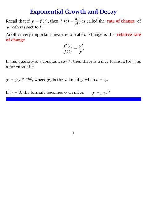
<strong>Exponential</strong> <strong>Growth</strong> <strong>and</strong> <strong>Decay</strong><br />
Recall that if y = f(t), then f ′ (t) = dy<br />
dt<br />
y with respect to t.<br />
is called the rate of change of<br />
Another very important measure of rate of change is the relative rate<br />
of change<br />
f ′ (t)<br />
f(t)<br />
= y′<br />
y .<br />
If this quantity is a constant, say k, then there is a nice formula for y as<br />
a function of t:<br />
y = y0e k(t−t0) , where y0 is the value of y when t = t0.<br />
If t0 = 0, the formula becomes even nicer: y = y0e kt<br />
1
If k>0, so that y is increasing with t, we say that we have exponential<br />
growth .<br />
If k
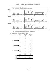
Some Real World Models:<br />
(1) Model #1: <strong>Growth</strong> of Bacterial Cultures<br />
It is known that under certain conditions a population of bacteria grow<br />
at a constant relative rate.<br />
The st<strong>and</strong>ard equation to represent this is<br />
P(t) = P(0)e kt , where P(0) is the population at time 0, <strong>and</strong> k is a constant<br />
that depends on the type of bacteria <strong>and</strong> its environmental conditions.<br />
Usually, this problem arises in a context where the population value is<br />
measured at two different points in time, <strong>and</strong> it is required to use this<br />
information to predict the population values at other times.<br />
In other words, two Data Points (t1,P1) <strong>and</strong> (t2,P2) are given, <strong>and</strong> one<br />
wishes to find the curve P(t) = P(0)e kt that passes through them.<br />
3
The simplest of such problems are those where the initial value of the<br />
population is given.<br />
Example: A bacteria culture starts with 4000 bacteria, <strong>and</strong> in 3 hours<br />
has grown to 7000.<br />
(1) Find a formula for the amount of bacteria after t hours.<br />
(2) How long will it take the population to double?<br />
(3) How long will it take the population to grow by a factor of 10?<br />
Solution: We have P(0) = 4000, <strong>and</strong> P(3) = 7000.<br />
We know that the population function satisfies the equation P(t) = P(0)e kt ,<br />
<strong>and</strong> since we have P(0) = 4000, we have P(t) = 4000e kt .<br />
We need to find k, so we use the other Data Point:<br />
P(3) = 7000 = 4000e k(3) = 4000e 3k .<br />
We must solve for k:<br />
We have 7000 = 4000e 3k ,so 7000<br />
4000 = e3k or 7<br />
4<br />
4<br />
= e3k
Taking natural logarithms, we have:<br />
ln 7<br />
4 = ln e3k = 3k, sok =<br />
<strong>and</strong> thus<br />
ln 7<br />
4<br />
3<br />
P(t) = 4000e kt = 4000e ln 7 4<br />
3 t = 4000<br />
t<br />
7 3<br />
4<br />
so now we have the desired formula for P(t).<br />
There are still two unanswered questions:<br />
(2) How long will it take the population to double?<br />
Since P(0) = 4000, we need to find the value of t for which P(t) = 8000,<br />
so we solve the equation:<br />
8000 = 4000e ln 7 4<br />
3 t for t:<br />
2 = e ln 7 4<br />
3 t<br />
5
7<br />
ln 4<br />
ln 2 =<br />
3 t<br />
<br />
3ln2= ln 7<br />
<br />
4<br />
t = 3ln2<br />
ln 7<br />
4<br />
t<br />
= 3ln2<br />
ln 7 − ln 4<br />
≐ 3.71<br />
This number is called the doubling time of an exponential growth model,<br />
<strong>and</strong> is denoted by T2.<br />
For a growth equation y = y0e kt , we have T2 =<br />
6<br />
ln 2<br />
k .
(3) How long will it take the population to grow by a factor of 10?<br />
Since P(0) = 4000, we need to find the value of t for which P(t) = 40000,<br />
so we solve the equation:<br />
10000 = 4000e ln 7 4<br />
3 t for t:<br />
10 = e ln 7 4<br />
3 t<br />
7<br />
ln 4<br />
ln 10 =<br />
3 t<br />
<br />
3ln10= ln 7<br />
<br />
4<br />
t = 3ln10<br />
ln 7<br />
4<br />
t<br />
= 3ln10<br />
ln 7 − ln 4<br />
This number is called the magnitude growth time of an exponential<br />
growth model, <strong>and</strong> is denoted by T10.<br />
For a growth equation y = y0e kt , we have T10 =<br />
7<br />
ln 10<br />
k .
Model #2: Radioactive <strong>Decay</strong><br />
It is known that radioactive elements decay at a rate proportional to the<br />
amount of the element present: in other words, the relative rate of change<br />
is constant, <strong>and</strong> negative.<br />
For example, radium-226 decays in such a way that half of it disappears<br />
every 1590 years. The decay equation<br />
y(t) = y0e kt must therefore satisfy 1<br />
2 y0 = y0e k(1590) so we can solve for<br />
k by eliminating y0 <strong>and</strong> taking logarithms:<br />
1<br />
= e1590k<br />
2<br />
<br />
1<br />
ln = ln 1 − ln 2 =−ln 2 = 1590k<br />
2<br />
so<br />
ln 2<br />
k =−<br />
1590 ≐−0.0004359<br />
8
Many people prefer to have the constant k positive, so they would start<br />
with the decay equation in the form<br />
y(t) = y0e −kt .<br />
In either case, the resulting model equation is<br />
ln 2<br />
−<br />
y(t) = y0e 1590t t<br />
−<br />
= y02 1590<br />
Note that it is easier to underst<strong>and</strong> the model’s equation when it is written<br />
in terms of powers of 2, rather than powers of e. It is essential that<br />
the student be able to move easily from one form to another. The number<br />
1590 is called the half-life of the decaying element, <strong>and</strong> is denoted<br />
by T 1 or T0.5.<br />
2<br />
If the decay equation is y(t) = y0e −kt ,(k>0), then we have T 1<br />
2<br />
= ln 2<br />
k .<br />
The length of time it takes an element to decay to one-tenth of its original<br />
value is called the magnitude decay time , denoted by T 1 or T0.1 <strong>and</strong><br />
10<br />
is related to k(> 0) by T 1 =<br />
10<br />
ln 10<br />
k .<br />
9
The General Problem<br />
Suppose we are told that a quantity y varies with time t at a constant<br />
relative rate of change, <strong>and</strong> we are given two data points (t1,y1) <strong>and</strong><br />
(t2,y2), from which we are to construct a model growth or decay equation<br />
which is then to be used to determine the doubling time or half-life <strong>and</strong><br />
the magnitude growth or decay time.<br />
Since we have two readings, we can insert then into the equation<br />
y(t) = y0e kt<br />
<strong>and</strong> get two data equations in the two unknown constants y0 <strong>and</strong> k:<br />
y1 = y0e kt1 <strong>and</strong> y2 = y0e kt2 .<br />
10
Taking the ratios of the two equations, we get<br />
y2<br />
y1<br />
= y0e kt2<br />
= ek(t2−t1)<br />
y0ekt1 <strong>and</strong> on taking logarithms we have<br />
<br />
y2<br />
ln = ln y2 − ln y1 = k(t2 − t1) so<br />
y1<br />
k = ln y2 − ln y1<br />
t2 − t1<br />
We can now use this in the first data equation to find the remaining unknown<br />
constant y0:<br />
y1 = y0e kt1 = y0e<br />
y0 = y1e − ln y2−ln y1 t2−t t1<br />
1<br />
ln y2−ln y1 t2−t t1<br />
1 ,so<br />
11
If we now put these values in the model equation,<br />
y(t) = y0e kt ,weget<br />
y(t) = y1e − ln y2−ln y1 ln y<br />
t2−t t1<br />
2−ln y1 1<br />
t e 2−t t<br />
1<br />
or<br />
y(t) = y1e<br />
ln y2−ln y1 t2−t (t−t1)<br />
1 = y1<br />
We could just as easily derive<br />
y(t) = y2<br />
y1<br />
y2<br />
t−t 2<br />
t 1 −t 2<br />
y2<br />
y1<br />
t−t 1<br />
t 2 −t 1<br />
The advantage of these two formulas is that is easy to check that they<br />
pass through the given data points.<br />
Of course, when doing practical calculations, these equation should, <strong>and</strong><br />
often must, be converted to base e <strong>and</strong> natural logarithm format.<br />
12
Model#3 Newton’s Law of Temperature Change<br />
Newton’s Law of Temperature Change says that the rate of change of<br />
the temperature of an object is directly proportional to the difference between<br />
its temperature, <strong>and</strong> the temperature of its surroundings, called<br />
the ambient temperature.<br />
Industrial applications of this model are plentiful: any situation which<br />
requires the heating or cooling of significant quantities of materials is<br />
modeled by this law. Examples are found in steel mills, large bakeries,<br />
chemical complexes, especially breweries, etc. It is also used by metallurgical<br />
engineers in the tempering of metal products.<br />
13
The Model<br />
We will let the temperature of the object be T(t), <strong>and</strong> since this will tend<br />
to the ambient temperature as t →∞, we will denote the ambient temperature<br />
by T∞.<br />
We will also denote the initial temperature T(0) by T0.<br />
It is important to notice that the temperature T(t) does not have a constant<br />
proportional rate of change:<br />
it is the function D(t) = T(t)− T∞ that satisfies<br />
D ′ (t)<br />
=−k for some constant k>0.<br />
D(t)<br />
We therefore have D(t) = D(0)e −kt = (T0 − T∞)e −kt , or, converting to<br />
expressions involving T(t) only:<br />
T(t)− T∞ = (T0 − T∞)e −kt<br />
or<br />
T(t) = T∞ + (T0 − T∞) e −kt = T∞<br />
<br />
1 − e −kt<br />
+ T0e −kt<br />
14
The Real World<br />
If we are lucky, we will know the initial temperature T0 <strong>and</strong> the ambient<br />
temperature T∞.<br />
We may, for example, want to cook a turkey, which we have brought home<br />
from the butcher thawed <strong>and</strong> at a temperature of 5 ◦ C. Leaving it in the<br />
kitchen sink, where the temperature is 20 ◦ C, while we prepare the stuffing,<br />
we observe that its temperature increases by 1 ◦ C in the 30 minutes<br />
it takes us to prepare the stuffing <strong>and</strong> to stuff the turkey. Our cookbook<br />
tells us to cook the turkey at an oven temperature of 180 ◦ C. If the turkey<br />
is considered to be cooked when it has reached the temperature of 85 ◦ C,<br />
how long will it take to cook the turkey?<br />
15
Solution:<br />
Phase I:Pre-Oven<br />
Before the turkey is in the oven, we have T0 = 5 <strong>and</strong> T∞ = 20, <strong>and</strong> we<br />
also have T(30) = 6, so we can solve for k:<br />
<br />
T(30) = T∞ 1 − e −k(30)<br />
+ T0e −k(30) <br />
= 6 = 20 1 − e −k(30)<br />
+ 5e −k(30)<br />
6 = 20 − 20e −30k + 5e −30k = 20 − 15e −30k<br />
−14 =−15e −30k<br />
e −30k = −14<br />
−15<br />
<br />
14<br />
−30k = ln<br />
15<br />
k =<br />
ln 14 − ln 15<br />
−30<br />
= ln 15 − ln 14<br />
30<br />
≐ 0.0022997<br />
16
Phase II:In the Oven<br />
When we put the turkey in the oven, we have T0 = 6, <strong>and</strong> T∞ = 180, so<br />
the temperature at time t will be<br />
<br />
T(t) = T∞ 1 − e −kt<br />
+ T0e −kt <br />
<br />
ln 15−ln 14<br />
ln 15−ln 14<br />
−<br />
= 180 1 − e 30 t −<br />
+ 6e 30 t<br />
=<br />
180 − 174e<br />
ln 15−ln 14<br />
− 30 t<br />
We have to find the time t when this equals 85:<br />
85 = 180 − 174e<br />
ln 15−ln 14<br />
− 30<br />
− ln 15−ln 14<br />
t if<br />
−95 =−174e 30 t<br />
if<br />
−95<br />
−174<br />
<br />
95 ln 15 − ln 14<br />
ln =− t if<br />
174<br />
30<br />
ln 15 − ln 14<br />
ln 95 − ln 174 =− t if<br />
30<br />
ln 95 − ln 174<br />
30 = t if<br />
−(ln 15 − ln 14)<br />
ln 15−ln 14<br />
= e− 30 t<br />
if( taking logarithms)<br />
17
ln 174 − ln 95<br />
t = 30<br />
ln 15 − ln 14<br />
or about 4.4 hours.<br />
≐ 300.6051784<br />
0.0689929<br />
Three Temperature Readings<br />
≐ 263 minutes<br />
It sometimes happens that three temperature readings (t1,T1), (t2,T2),<br />
<strong>and</strong> (t3,T3) are taken, <strong>and</strong> it is desired to use them to find the complete<br />
equation of the temperature of the object being studied.<br />
We get three equations in the three unknown constants T0, T∞, <strong>and</strong> k:<br />
T1 = T∞ + (T0 − T∞) e −kt1<br />
T2 = T∞ + (T0 − T∞) e −kt2<br />
T3 = T∞ + (T0 − T∞) e −kt3<br />
18
Witout some extra information these equations are usually impossible<br />
to solve. It is usually easy to arrange for the times between the three<br />
measurements to be equal, say to ∆t. Then we have t2 = t1 + ∆t <strong>and</strong><br />
t3 = t1 + 2∆t, <strong>and</strong> it is possible to eliminate T0 <strong>and</strong> k:<br />
T1 − T∞ = (T0 − T∞) e −kt1<br />
T2 − T∞ = (T0 − T∞) e −k(t1+∆t)<br />
T3 − T∞ = (T0 − T∞) e −(kt1+2∆t)<br />
(A) T1 − T∞<br />
T0 − T∞<br />
(B) T2 − T∞<br />
T0 − T∞<br />
(C) T3 − T∞<br />
T0 − T∞<br />
= e −kt1<br />
= e −k(t1+∆t)<br />
= e −k(t1+2∆t)<br />
Now we divide equation (B) by equation (A) <strong>and</strong> equation (C) by equation<br />
(B):<br />
19
T2 − T∞<br />
T1 − T∞<br />
T3 − T∞<br />
T2 − T∞<br />
so we have<br />
T2 − T∞<br />
T1 − T∞<br />
= e−k(t1+∆t)<br />
e −kt1<br />
= e−k∆t<br />
= e−k(t1+2∆t)<br />
= e−k∆t<br />
e−k(t1+∆t) = T3 − T∞<br />
T2 − T∞<br />
Note that T0 has disappeared. Simplifying, we get:<br />
(T2 − T∞)(T2 − T∞) = (T1 − T∞)(T3 − T∞)<br />
or T 2 2 − 2T2T∞ + T 2 ∞ = T1T3 − (T1 + T3)T∞ + T 2 ∞<br />
or (T1 − 2T2 + T3)T∞ = T1T3 − T 2 2<br />
or T∞ = T1T3 − T 2 2<br />
T1 − 2T2 + T3<br />
20
We now use this to find:<br />
e −k∆t = T2 − T1T3−T 2 2<br />
T1−2T2+T3<br />
T1 − T1T3−T 2 2<br />
T1−2T2+T3<br />
T2(T1 − 2T2 + T3) − (T1T3 − T 2 2 )<br />
T1(T1 − 2T2 + T3) − (T1T3 − T 2 =<br />
2 )<br />
=<br />
T1T2 − 2T 2 2 + T2T3 − T1T3 + T 2 2<br />
T 2 1 − 2T1T2 + T1T3 − T1T3 + T 2 2<br />
=<br />
T1T2 − T 2 2 + T2T3 − T1T3<br />
T 2 1 − 2T1T2 + T 2 =<br />
2<br />
T2(T1 − T2) + T3(T2 − T1)<br />
(T1 − T2) 2<br />
=<br />
(T3 − T2)(T2 − T1)<br />
(T2 − T1) 2<br />
= T3 − T2<br />
T2 − T1<br />
If this quantity is not positive there is no mathematical solution, which<br />
should tell us that there is a problem with the data or with the model.<br />
If this quantity is positive but is greater than 1 there is also a problem,<br />
because this would tell us that the temperature is going to tend to ±∞!<br />
21
Using e −k∆t = T3 − T2<br />
we can solve explicitly for k:<br />
T2 − T1<br />
<br />
T3 − T2<br />
−k∆t = ln<br />
= ln(T3 − T2) − ln(T2 − T1)<br />
T2 − T1<br />
k = ln(T2 − T1) − ln(T3 − T2)<br />
∆t<br />
Next we substitute the values of k <strong>and</strong> T∞ into equation (A) to find T0:<br />
(A) T1 − T∞<br />
T0 − T∞<br />
T1 − T1T3−T 2 2<br />
T1−2T2+T3<br />
T0 − T1T3−T 2 2<br />
T1−2T2+T3<br />
= e −kt1 becomes<br />
= e −( ln(T2−T1 )−ln(T3−T2 )<br />
∆t )t1 or<br />
T1(T1 − 2T2 + T3) − (T1T3 − T 2 2 )<br />
T0(T1 − 2T2 + T3) − (T1T3 − T 2 = eln<br />
2 )<br />
<br />
T3−T2 t1<br />
T2−T1 ∆t or<br />
T 2 1 − 2T1T2 + T1T3 − T1T3 + T 2 2 )<br />
T0(T1 − 2T2 + T3) − (T1T3 − T 2 <br />
T3 − T2<br />
=<br />
2 ) T2 − T1<br />
22<br />
t 1<br />
∆t<br />
or
(T1 − T2) 2<br />
T0(T1 − 2T2 + T3) − (T1T3 − T 2 <br />
T3 − T2<br />
=<br />
2 ) T2 − T1<br />
(T1 − T2) 2<br />
<br />
T3 − T2<br />
T2 − T1<br />
(T1 − T2) 2<br />
<br />
T3 − T2<br />
T0 = (T1 − T2) 2<br />
T2 − T1<br />
−t 1<br />
∆t<br />
−t 1<br />
∆t<br />
t 1<br />
∆t<br />
or<br />
= T0(T1 − 2T2 + T3) − (T1T3 − T 2 2 ) or<br />
+ (T1T3 − T 2 2 ) = T0(T1 − 2T2 + T3) or<br />
<br />
T3−T2<br />
T2−T1<br />
−t1 ∆t<br />
+ (T1T3 − T 2 2 )<br />
T1 − 2T2 + T3<br />
We now insert these values into the formula for T(t):<br />
T(t) = T∞ + (T0 − T∞) e −kt<br />
becomes:<br />
T(t) = T1T3 − T 2 2<br />
T1 − 2T2 + T3<br />
+<br />
(T1 − T2) 2<br />
T1 − 2T2 + T3<br />
23<br />
T3 − T2<br />
T2 − T1<br />
t−t 1<br />
∆t
It is often convenient to change the notation: we let<br />
∆T1 = T2 − T1 <strong>and</strong> ∆T2 = T3 − T2, we get T2 = T1 + ∆T1, <strong>and</strong> T3 =<br />
T1 + ∆T1 + ∆T2, so<br />
T∞ = T1T3 − T 2 2<br />
T1 − 2T2 + T3<br />
= T1(T1 + ∆T1 + ∆T2) − (T1 + ∆T1) 2<br />
∆T2 − ∆T1<br />
T 2 1 + T1∆T1 + T1∆T2 − (T 2 1 + 2T1∆T1 + ∆T 2 1 )<br />
T1 −<br />
∆T 2 1<br />
∆T2 − ∆T1<br />
e −k∆t = T3 − T2<br />
T2 − T1<br />
(∆T1) 2<br />
∆T2 − ∆T1<br />
= ∆T2<br />
∆T1<br />
∆T2<br />
∆T1<br />
−t <br />
1<br />
∆t<br />
− 1<br />
T0 = T1 +<br />
∆T2 − ∆T1<br />
⎡<br />
2 <br />
(∆T1) ∆T2<br />
T(t) = T1 + ⎣<br />
∆T2 − ∆T1 ∆T1<br />
t−t 1<br />
∆t<br />
− 1⎦<br />
24<br />
⎤<br />
=<br />
= T1(∆T2 − ∆T1) − ∆T 2 1<br />
∆T2 − ∆T1<br />
=
Model # 4 Dilution of Chemicals<br />
Suppose a tank contains a volume V litres of fluid with a concentration<br />
c0 of chemical X, <strong>and</strong> that there is an inflow into the tank of the fluid at<br />
the rate r litres per minute with a conentration level of cin of chemical X.<br />
Assumung that the tank is continuously <strong>and</strong> thoroughly mixed, so that<br />
the concentration is uniform throughout the tank, <strong>and</strong> that fluid is drawn<br />
off at the same rate, so that the volume remains constant.<br />
26
Clearly the concentration will tend to cin, <strong>and</strong> the amount of chemical X<br />
in the tank will therefore tend to cinV . Let x(t) be the amount of chem-<br />
ical X, <strong>and</strong> let cout(t) be the concentration of chemical X in the tank at<br />
time t. We have cout(t) = x(t)<br />
V<br />
x ′ <br />
kg<br />
(t) = cin<br />
ℓ<br />
<br />
cin − x(t)<br />
=<br />
V<br />
kg<br />
, <strong>and</strong><br />
ℓ<br />
<br />
− cout(t) r ℓ<br />
min =<br />
<br />
kg<br />
cin<br />
ℓ<br />
r kg<br />
min<br />
Next we let D(t) = x(t) − cinV , so that<br />
D ′ (t) = x ′ <br />
cin − x(t)<br />
(t) =<br />
V<br />
r kg<br />
min<br />
or, discarding units for the moment,<br />
D ′ (t)<br />
D(t) =−r<br />
V ,<br />
r<br />
−<br />
which has solution D(t) =D(0)e V t .<br />
− x(t)<br />
V<br />
=−D(t) r<br />
V<br />
27<br />
kg<br />
min<br />
<br />
kg<br />
r<br />
ℓ<br />
ℓ<br />
min
This can now be converted into expressions for x(t) <strong>and</strong> c(t):<br />
We have D(0) = x(0) − cinV = c0V − cinV = (c0 − cin)V ,so<br />
r<br />
−<br />
D(t) = (c0 − cin)V e V t , <strong>and</strong> thus<br />
r<br />
−<br />
x(t) − cinV = (c0 − cin)V e V t , giving us<br />
r<br />
−<br />
x(t) = cinV + (c0 − cin)V e V t <br />
r<br />
−<br />
= cin + (c0 − cin)e V t<br />
V <strong>and</strong><br />
r<br />
−<br />
c(t) = cin + (c0 − cin)e V t .<br />
28