USLE-M

USER’S GUIDE
DRAFT
October 2005
AGNPS – UM Version 4.02
Agricultural Non Point Source Pollution Model
using the
USLE-M
(not to be confused with the MUSLE)
P.I.A. Kinnell
University of Canberra
Canberra
AUSTRALIA
AGNPS-UM User’s Guide I

Disclaimer
The software to which this User’s Guide applies is used entirely at the user’s own risk.
While every effort has been made to ensure that the software is error free, the
software is used by the recipient upon the express understanding that the developer
makes no warranties, expressed or implied, concerning the accuracy, completeness,
reliability or suitability for any one purpose, and that the developer shall be under no
liability to any person by reason of any use made thereof.
Contents
page
USLE-M Theory
USLE-M erosivity factor 1
USLE-M soil erodibility 3
USLE-M Crop and crop management factor 4
Predicting erosion via the USLE-M 5
The USLE-M lite (uses USLE C and P factors directly) 7
Caution (USLE-M lite NOT direct replacement for USLE-M) 8
AGNPS-UM software 9
Installing and running the software 10
Erosion model options 11
Graphic output 13
Output data files 13
Example data 14
Literature 14
Erosion on a dry catchment/watershed – AGNPS-UM takes account of moisture status
.
AGNPS-UM User’s Guide II

AGNPS - UM
AGNPS, the Agricultural Non Point Source Pollution model, was developed in the USA to
predict the effect of land use on the quality of water discharged from catchments or
watersheds. It is an event based model and uses the Universal Soil Loss Equation (USLE)
to predict erosion within grid cells on hillsides. The USLE was not designed to predict
event erosion. A modification of the USLE called the USLE-M can do this better. AGNPS-
UM uses the USLE-M instead of the USLE.
USLE-M theory
The USLE-M is a variant of the Universal Soil Loss Equation (USLE) and the Revised
version of it (RUSLE). The USLE is an empirical model that predicts average annual
erosion (A) in terms of 6 factors;
A = R K L S C P (1)
where R is the rainfall-runoff factor, K is the soil erodibility factor, L is the slope length
factor, S is the slope gradient factor, C is the crop and crop management factor and P is the
supporting practices factor. The R factor is the annual average value of the event erosivity
factor (Re) where
Re = E I30 (2)
where E is the total kinetic energy of the rainfall event and I30 is the maximum 30-minute
rainfall intensity (maximum intensity using a 30-minute time frame).
USLE-M event erosivity factor – the QREI30 index
Although the USLE was not designed to predict event erosion, it follows from Eqs. 1 and 2
that
Ae = [E I30]e Ke L S Ce Pe (3)
where the subscript e indicates factor values that vary between rainfall events. The USLE-
M uses QREI30, where QR is the runoff ratio for the area being considered, instead of the
EI30 for the event erosivity factor.
Because the USLE is an empirical model, changing the event erosivity index from EI30 has
consequences. The soil erodibility factor must be changed because it has units of soil loss
per unit of the erosivity factor. The crop and support practice factors must also be changed
to account for the movement of the runoff effect which they normally deal with to the
erosivity factor. Consequently, the USLE-M is given by
Ae = [QR E I30]e KeUM L S CeUM PeUM (4)
where the subscript UM indicates factors that differ in value from the factors used in the
USLE.
While the USLE-M is an empirical model, the QREI30 index has a physical basis. The
sediment discharged with runoff is given by the product of runoff and sediment
AGNPS-UM User’s Guide 1

predicted soil loss (t/ha)
concentration and the QREI30 index results from considering that the sediment
concentration for an event is dependent the energy per unit quantity of rain and a measure
of the maximum rainfall intensity since a large proportion of the runoff is generated during
time when the rainfall intensity is high. The energy per unit quantity of rain is given by E
divided by rainfall amount and I30 is a measure of the maximum rainfall intensity. Thus
ReUM = Qe (E / event rainfall amount) I30 (5)
where Qe is the amount of runoff for the event. However
QR = Qe / event rainfall amount (6)
so that
ReUM = QR E I30 (7)
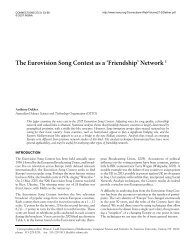
On a bare fallow area (Ce = CeUM = 1) with cultivation up and down the slope (Pe = PeUM =
1), event erosion is give by
Ae( CeUM = PeUM = 1) = b [QR E I30]e (8)
where b = KeUM L S. Figure 1 provides a comparison between Eq. 8 and the USLE
equivalent
Ae( Ce = Pe = 1) = b [E I30]e (9)
where b = Ke L S.
100
10
1
0.1
0.01
R e = EI 30
0.01 0.1 1 10 100
observed soil loss (t/ha)
Eff ln = 0.084
Figure 1. Relationships between observed and predicted event soil loss for plot 10
(bare fallow) in experiment 1 at Morris, MN when predicted = bRe where Re is EI30
and QREI30. Effln is the Nash-Sutcliffe (1970) efficiency factor for the ln transforms of
the data and reflects the amount of variation from the 1:1 lines shown in these figures.
NB. This analysis takes no account of short term variations in K or KUM.
AGNPS-UM User’s Guide 2
predicted soil loss (t/ha)
100
10
1
0.1
0.01
R e = Q REI 30
0.01 0.1 1 10 100
observed soil loss (t/ha)
Eff ln = 0.738

The runoff and soil loss plot used in this comparison is part of the USLE data base. The
total loss from the plot was 374 t ha -1 from 80 events over 10 years. The top 5 events
produced 177 t ha -1 . The USLE (Eq. 9) predicted 123 t ha -1 (-31% error) while the USLE-M
(Eq. 8) predicted 164 t ha -1 (-7% error). The 10 events producing the lowest soil loss
contributed 0.83 t ha -1 . The USLE predicted 25 t ha -1 for these events, the USLE-M 1.12 t
ha -1 . The Nash-Sutcliffe (1970) efficiency factor (Effln) provides a measure of a model’s
performance. A value of 1.0 is achieved by the perfect model. Effln for the QREI30 index is
0.734 while the EI30 index gives 0.084. A value of zero means that the model predicts no
better than if the mean of the independent variable (EI30 or QREI30) is used.
USLE-M Soil Erodibility (KUM)
A noted above, the soil erodibility factor for the USLE-M (KUM) differs from that of the
USLE because the soil erodibility factor in both models has units of soil loss per unit of the
erosivity factor. Because Ce = CeUM = Pe = PeUM = 1.0 when the area being eroded is bare
fallow with cultivation up and down the slope, the annual average value of the USLE-M
soil erodibility factor can be determined from data such as shown in Figure 1. The general
equation for determining average annual soil erodibility for any given event erosivity index
(Xe) is
N
ΣAe1
e=1
K(Xe) = ____________ (10)
N
Σ Xe
e=1
where Ae1 is event soil loss on what is called “the unit plot”, bare fallow with cultivation up
and down the slope on an 22.13 m long slope with a gradient of 9 %, and N is the number
of events used to determine K(Xe). Since the USLE-M uses the USLE L and S factor
values, event soil losses obtained on areas of bare fallow with cultivation up and down the
slope that are not 22.13 m long on a 9 % slope can be converted to unit plot values using
the USLE or the RUSLE L and S factors.
L = (λ / 22.13 ) m (11)
where λ is the slope length and m is a power that is related to the ratio of rill and interrill
erosion. In the USLE
m = 0.6 slope > 10% (12a)
m = 0.5 5 - 10% (12b)
m = 0.4 3 - 5% (12c)
m = 0.3 1 - 3% (12d)
m =.0.2 < 1% (12e)
In the RUSLE,
m = β / ( 1+ β) (13)
where, for soil that is moderately susceptible to rilling
AGNPS-UM User’s Guide 3

β = (sin θ / 0.0896) / [3.0 (sin θ ) 0.8 + 0.56] (14)
where θ = angle to horizontal.
The slope gradient factor (S) for the USLE is given by
S = 65.4 sin 2 θ + 4.56 sin θ + 0.654 (15)
but was replaced by
S = 10.8 sin θ + 0.03 slopes < 9% (16a)
S = 16.8 sin θ - 0.50 slopes ≥ 9% (16b)
in the RUSLE because Eq. 15 overestimated erosion on high slope gradients.
USLE-M Crop and Crop Management (CUM)
As indicated in Eq. 4, the USLE-M Crop and Crop Management factor (CUM) values differ
from the USLE Crop and Crop Management factor (C) values because the runoff effect that
is included in C is moved to the erosivity factor when the erosivity factor is based on runoff
from the vegetated area. Table 1 shows annual average values of the Crop and Crop
Management factor for the USLE-M and the USLE for crops determined from erosion
experiments at various locations in the USA.
Table 1. Examples of CUM values for crops at various USA locations
Location Crop CUM CU CUM/CU CU/CUM
Bethany, Missouri alfalfa 0.008 0.002 4.0 0.250
corn 0.674 0.628 1.1 0.932
corn/meadow/wheat 0.188 0.106 1.8 0.564
Clarinda, Iowa corn 0.634 0.316 2.0 0.498
corn/oats/meadow 0.424 0.168 2.5 0.396
Guthrie, Oklahoma cotton 2.435 1.357 1.8 0.557
Bermuda grass 0.064 0.002 32.3 0.031
wheat/clover/cotton 0.913 0.344 2.7 0.377
LaCrosse, Wisconsin corn 0.527 0.469 1.1 0.890
Madison, S.Dakota corn(ploughed) 0.486 0.337 1.4 0.693
corn(mulch till) 0.384 0.250 1.5 0.651
Morris, Minnesota corn 0.520 0.434 1.2 0.835
meadow/corn/oats 0.046 0.010 4.6 0.217
Presque Isle, Maine potatoes 0.634 0.316 2.0 0.498
AGNPS-UM User’s Guide 4

These values were determined using
and
N
Σ Ae..c
e=1
C = ———————— (17)
N
LS K Σ (EI30)e
e=1
N
Σ Ae.c
e=1
CUM = ————————— (18)
N
LS KUM Σ (QREI30)e
e=1
where K and KUM were determined from data from bare fallow plots at the respective sites.
Predicting erosion via the USLE-M
While the USLE is an empirical model whose factor values were originally determined
from erosion experiments, procedures for determining factor values from soil, crop and
management data have been developed to facilitate the prediction of erosion using the
USLE. For example, an equation was developed to calculate soil erodibility in the USLE
for soils that contain less than 70% silt in the USA ,
K = [2.1 10 -4 (12-OM) M 1.14 + 3.2(s-2) + 2.5(p-3)]/100 (19)
where K is in customary US units, OM is percent organic matter, M depends on the soil
texture, s is soil structure class, and p is permeability. Other equations exist for soils in
other geographic locations such as Hawaii.
The USLE-M soil erodibility factor is greater than the USLE soil erodibility factor because
of the inclusion of QR, the runoff ratio, in the event erosivity index. KUM is related to K via
the inverse of the runoff ratio for bare fallow and cultivation up and down the slope (QR1)
through a coefficient (kKUM)
so that
N
Σ (EI30)e
e=1
kK.UM = ————— (20)
N
Σ (QR1EI30)e
e=1
KUM = kK.UM K (21)
AGNPS-UM User’s Guide 5

In most cases, soil erodibility is considered to relatively constant in comparison to
variations in C and P so that, in most cases,
can be used.
KUMe = KUM (22)
The gross runoff ratio for runoff producing events (GRRrope) is given
N
Σ Qe.
e=1
GRRrope = ——— (23)
N
Σ Be
e=1
where Be is event rainfall and data obtained from the USLE runoff and soil loss plot data
base shows that kKUM can be estimated by
kK.UM = (GRRrope) - 0.79 (24)
Given an ability to predict event runoff from event rainfall, it is possible to determine
GRRrope and convert K to KUM.
CUM values can be calculated from C values through
where
As with kK.UM,
CUM = C kC.UM / kK.UM (25)
N
Σ (EI30)e
e=1
kC.UM = ————— (26)
N
Σ (QREI30)e
e=1
kC.UM = (GRRrope) - 0.79 (27)
when GRRrope is known for the vegetated condition.
A similar approach can be used to determine PUM from P.
Theortically, it follows from Eqs. 20, 25 and 26 that event values of CUM and PUM can be
determined from event values of C and P by multiplying the relevant USLE factor values
by ratio of QR1e to QRe when QRe > 0. However, that assumes that the runoff effect on
erosion under non unit plot conditions is considered correctly within the determination of
Ce and Pe values. That assumption may not be correct given that procedures for determining
short term values of C and P may subjective and not give proper consideration as to how
AGNPS-UM User’s Guide 6

unoff and sediment concentration influence erosion. For example, the USLE/RUSLE uses
period (fortnightly) C values and it is logical to suggest that Ce values during a fortnightly
period are equal to the period C value. However, this would produce CeUM values that vary
between events with the ratio of QR1e to QRe where as the effect of the crop on sediment
concentration should remain relatively constant during that period. Appropriate rules for
determining CeUM values from crop morphology and management have yet to be developed.
The USLE-M lite
Procedures exist for determining short term values of C and P in the RUSLE but similar
procedures have yet to be developed to determine CeUM and PeUM. However, despite Eq. 4,
an approach does exist that enables short term values of C and P to be used directly when
the QREI30 is used as the event erosivity index.
The USLE/RUSLE model is based on the prediction of erosion for the unit plot condition
(22.1m long slope, 9% gradient, bare fallow with cultivation up and down the slope) and
the L, S, C and P factors are ratios with respect to the unit plot. Thus, the approach is in
effect a two staged one; the prediction of erosion for the unit plot condition where
A1 = R K (28)
where A1 is the annual average erosion on the unit plot, R is the annual average erosivity
factor and K is the average annual soil erodibility, followed by
A = A1 L S C P (29)
where A is the average annual erosion on an area that differs from the unit plot is some
way. In the context of a rainfall event, these two equations become
and
A1e = Re Ke (30)
Ae = A1e L S Ce Pe (31)
where Re = EI30. As indicated above, KUMe ≠ Ke, CUMe ≠ Ce, PUMe ≠ Pe. However, CUMe ≠ Ce
and PUMe ≠ Pe only applies when the runoff values used to determine QR in Eq. 4 are those
associated with an area that is vegetated and cultivation is not up and down the slope. Thus,
if the QREI30 index is used to predict erosion for the bare fallow cultivation up and down
the slope condition (C = P = 1), then
Ae(C = P = 1) = k KUMe [QR1EI30]e (32)
where k = LS, and values for C and P generated by the USLE or the RUSLE can be used to
give
Ae = [QR1EI30]e KUMe L S Ce Pe (33)
where QR1 is the runoff ratio for the bare fallow and cultivation up and down the slope
condition. The procedures for determining short term values for C and P in the RUSLE
AGNPS-UM User’s Guide 7

documentation (Renard et al., 1997) can thus be used as a guide to determining Ce and Pe
values for use in Eq. 31.
The model described by Eq. 33 is called the USLE-M lite to distinguish it from that
described by Eq. 4.
Caution
The USLE-M lite is NOT a direct replacement for the USLE-M in respect to
modelling event erosion.
The USLE-M lite, like the USLE, is based on the assumption that erosion occurs when C ≠
1 and P ≠ 1 whenever erosion occurs when C = 1 and P = 1. Normally, there are many
occasions where erosion occurs on a bare fallow area but not on a vegetated one, and there
may be occasions where erosion occurs on a vegetated area but not on a bare fallow area.
Figure 2 shows the result predicting event soil losses by multiplying observed event soil
losses from an adjacent bare fallow plot by period C values for conventional corn at
Clarinda, Iowa over a 7 year period.
predicted event soil loss (T/A)
100.000
10.000
1.000
0.100
0.010
0.0001 0.0010 0.0100 0.1000 1.0000 10.0000 100.0000
observered event soil loss + 0.0001 (T/A)
Figure 2. Relationship between event soil losses predicted by multiplying event soil
losses from a nearby bare fallow plot by RUSLE period Soil Loss Ratios (fortnightly C
factor values) and event soil losses observed for conventional corn at Clarinda, Iowa
plus 0.0001 tons acre-1 to enable predicted losses to be displayed when observed losses
are zero.
The total observed and predicted amounts over the 7 years were in close agreement (130
tons acre -1 observed, 131 tons acre -1 predicted) but 12 % of the predicted amount was
contributed by events that produced zero erosion on the cropped plot. Because the USLE-M
event erosivity index is based on runoff from areas where C ≠ 1 and P ≠ 1, the USLE-M is
more appropriately applied to modelling event erosion than the USLE-M lite.
AGNPS-UM User’s Guide 8

AGNPS-UM software
The AGNPS-UM software predicts erosion in customary US units (tons/acre) in grid cells
within a catchment or watershed given 3 ascii GIS files and a USLE/USLE-M attribute data
file. The GIS files are grid cell files for elevation, soils and land use and the user needs to
know the grid cell coordinates of the catchment or watershed outlet and the cell size
(metres). The cell size should be of the order of 100 m or less. The acsii files can have a
GRASS, ARCH/INFO or MAPINFO format. The ascii files are used in conjunction with
TOPAZ (http://duke.usask.ca/~martzl/topaz) to identify the catchment or watershed
boundary, generate an artificial stream network, as well as determine grid cell slope
gradient and flow direction using the D8 method.
The software can handle grids of up to 1000 by 1000 (1 million) cells. The restriction
of 32,000 cells that applies to the original AGNPS executables does not apply to the
AGNPS-UM software.
The USLE/USLE-M attribute data file is generated by the user to contain Ke, Ce, Pe values
for the USLE and KeUM, CeUM, PeUM values for the USLE-M for the relevant soils and
landuses. The units for these data are customary US units. Table 2 provides an example of
the USLE/USLE-M attribute data file.
Table 2. Example of the AGNPS/USLE-M data file
- Back Ck
Part of Chaffey Dam catchment
2.80 rain(inch)
62.0 EI30(100ft-ton-inch/A-h)
6 soils K texture CN bare ident
1 0.38 3 80 dummy clay
3 0.30 2 75 Alluvial
4 0.30 3 75 Black Earth
5 0.28 3 70 Krasnozem
6 0.38 2 85 Lithosols
7 0.40 1 80 Solodics
5 luses C P fert avN avP man's n s.cond COD ident
1 0.05 1.0 0 00 00 0.050 0.01 60 dummy = native pasture (outside)
3 0.003 1.0 0 00 00 0.050 0.01 60 undisturbed forest
5 0.05 1.0 0 00 00 0.050 0.01 60 native pasture
6 0.10 0.5 2 60 60 0.060 0.15 60 improved pasture
7 0.15 0.5 2 65 65 0.250 0.05 80 crop
6 soils Kum ident
1 0.50 dummy clay
3 0.47 Alluvial
4 0.40 Black Earth
5 0.37 Krasnozem
6 0.60 Lithosols
7 0.88 Solodics
5 luses Cum Pum CNadj ident
1 0.111 1.0 0.80 dummy = native pasture (outside)
3 0.03 1.0 0.70 undisturbed forest
5 0.111 1.0 0.80 native pasture
6 0.2 0.5 0.85 improved pasture
7 0.28 0.5 0.87 crop
USDA Curve Numbers (CN) are used for runoff prediction in AGNPS and CN values for
bare soil and cultivation up and down the slope are also entered into the USLE/USLE-M
attribute data file together with CN conversion coefficients which are used to convert CNs
for bare soil to CNs for the vegetated areas. Runoff prediction from vegetated areas is based
on the assumption that the ratio of CN vegetated to CN bare + cultivation up and down the
slope does not vary between soils. Event EI30 and rainfall amount are also entered via the
USLE/USLE-M attribute data file. In addition to the USLE/USLE-M attribute data inputs,
AGNPS-UM User’s Guide 9

the USLE/USLE-M attribute data file contains data normally associated with AGNPS such
as Manning’s n, data on fertilizer use and release etc. Users should consult the AGNPS
User Manual which can be obtained via http://www.sedlab.olemiss.edu/agnps/archives.html
in relation to the values for these data.
The software package contains set of example data files, bkckelev.dat (elevation),
bkckluse.dat (landuse), bkcksoil (soil) and bkckcat.dat (USLE/USLE-M attribute data).
Table 2 shows the contents of bkckcat.dat and agnps.dat. agnps.dat is the file that is used by
the software when generating the data input files that the AGNPS-UM software uses during
the calculation phase. The contents of agnps.dat can replaced by the contents of bkckcat.dat
or any other appropriate USLE/USLE-M attribute data file when necessary. agnps.dat can
contain global data that is not relevant to catchment or watershed being modelled. The
software will crash if relevant data is missing.
A facility exists in the software package to generate new agnps.dat files. However, it is
easier to edit existing ones. These files are space deliminated.
Installing and running the software package
The software package is contained in a .ZIP file which will set up the appropriate
directories/folders when the software is extracted using directory/folder names option is
flagged.
The program execution file is AGUMxxx.exe where xxx is the version number.
The operations of the program are controlled through a menu.
(1) Set up GIS and attribute files
(2) Generate grid cells and flow network
(3) Generate AGNPS input and output data files
(4) View catchment graphic
(5) Stitch GIS outputs into larger area
(6) END
(7) Information about running example
(1) Set up GIS and attribute files is the first step. When this step is invoked, the user
specifies the GIS files to be used by the program. The user needs to be aware of the format
of these files and ensure that they meet the format that the software will accept (GRASS,
ARCH/INFO, MAPINFO). Elevation data can be stored with various levels of precision.
The user will be asked to provide a factor that will convert the GIS elevation data to metres.
The software will respond with data on maximum and minimum elevations in metres and
the user can return to enter a new conversion factor if necessary. The user should note the
maximum and minimum elevations for use later. All three GIS files (elevation, landuse,
soils) must be nominated in response to selecting Set up GIS and attribute files unless they
have been dealt with previously. If a new set of landuses is the only change, then its GIS
file is the only one that needs to be processed.
AGNPS-UM User’s Guide 10

The facility to generate the agnps.dat file is included in Set up GIS and attribute files. As
noted earlier, the better option is to edit and store an existing one so that this facility may be
seldom used. If a new agnps.dat file is generated via Set up GIS and attribute files and
needs to be stored in case it gets overwritten, then the user will need to use Windows
facilities to do this.
(2) Generate grid cells and flow network causes TOPAZ to generate grid cells and
the flow network from the elevation file. During this process, the user has to enter data on
cell size, valid elevations ( recall maximum and minimum elevations given during Set up
GIS and attribute files), the grid cell coordinates of the outlet cell, and the critical source
area (CSA) in hectares for channel initiation. TOPAZ initiates a channel where ever the
upslope area exceeds the CSA.
(3 ) Generate AGNPS input and output data files gives the user the choice of a
number of models to run.
(1) The USLE with L via Desmet and Govers (1996)
(2) The USLE with L via Kinnell (2004)
(3) The USLE-M lite
(4) The USLE-M
(1) The USLE with L via Desmet and Govers (1996)
The L factor in the USLE is designed to work over an area whose length begins where
overland flow starts. A grid cell often is an area some distance downslope from where
runoff starts. In such circumstances, a grid cell receives runoff from upslope and the
erosion within that cell depends on the length of the cell and the effective length of the
upslope area. If the upslope area is rectangular and the same width as the cell, the slope
effect length of the upslope area is the same as the physical slope length. However, this is
not the case when the flow in through the upslope boundary of the cell comes from an area
with some other shape. According to Desmet and Govers (1996), the effective slope length
of the upslope area in all cases is given by the upslope area divided by the width of the
boundary over which the runoff flows which is the width of the cell. Consequently, for a
cell with coordinates i,j,
( Ai,j-in + D 2 ) m+1 - Ai,j-in m+1
Li,j = —————————— (32)
D m+2 xi,j m λ1 m
where Ai,j-in is the area (m 2 ) upslope of the cell, D is cell size (m), m is the coefficient used
in the calculation of L, x is a factor that depends on direction of flow with respect to the
orientation of the cell, and λ1 is the length of slope for the unit plot (22.13 m). The USLE
with L via Desmet and Govers (1996) uses Eq. 32 in the calculation of cell erosion.
(2) The USLE with L via Kinnell (2004)
With Eq. 32, if runoff does not enter from upslope, then Ai,j-in = 0 and Eq. 32 gives the
same value as Eq. 11. Thus, cells adjacent to the boundary of the catchment or watershed
AGNPS-UM User’s Guide 11

act essentially as isolated areas. However, it is possible that a cell somewhere in the
catchment or watershed may not produce any runoff across its downstream boundary
because it has a high infiltration capacity. Logically, Ai,j-in = 0 for the cell downslope of that
cell and that condition can be set whenever the runoff coefficient for the uppslope area
(QCi,j –in) is found to be zero. However, it is also logical to suggest that the effective upslope
area (Ai,j-in.eff ) is less than the physical area (Ai,j-in) whenever QCi,j-in is less than the runoff
coefficent of the area including the cell (QCi,j-all ) so that (Kinnell, 2005)
where
( Ai,j-in.eff + D 2 ) m+1 - Ai,j-in.eff m+1
Li,j = ————————————— (33)
D m+2 xi,j m λ1 m
Ai,j-in.eff = Ai,j-in QCe.i,j-in / QCe.i,j-all (34)
The USLE with L via Kinnell (2004) option calculates erosion using Eqs. 33 and 34.
(3) The USLE-M lite
Eqs. 33 and 34 are also fundamental to applying the USLE-M lite and the USLE-M to the
prediction of erosion in grid cells. When runoff is generated uniformly over an area,
QCe.i,j-all (Ai,j-in + D 2 ) m+1 - QCe.i,j-all Ai,j-in m+1
LUMe i,j = ————————————————— (35)
QRe.i,j-cell D m+2 xi,j m (22.13) m
where QRe.i,j-cell is the runoff ratio for the cell. QRe.i,j-cell is the ratio of the volume of water
discharged from the cell to the volume of rain water falling onto the cell. Because the
volume of water discharged from the cell includes runon from upslope, it can have values
greater than 1.0. QRe.i,j-cell occurs in Eq. 35 because the erosivity index for a cell is given by
the product of QRe.i,j-cell and EI30. Runoff coefficents are ratios of rain and runoff volumes
on the same area and consequently have values of 1.0 or less with Hortonian overland
flow.When considered in the context of Ai,j-in.eff determined by Eq 34, Eq. 35 becomes
QCe.i,j-all.eff (Ai,j-in.eff + D 2 ) m+1 - QCe.i,j-all.eff Ai,j-in.eff m+1
LUMe i,j = ——————————————————————— (36)
QRe.i,j-cell D m+2 xi,j m (22.13) m
In the case of the USLE-L lite, QCe.i,j-all.eff is the runoff coefficient for the area including the
cell when the whole area is considered to be bare fallow with cultivation up and down the
slope,
QCe.i,j-all.eff = [(QC1e.i,j-cell D 2 ) + (QC1e.i,j-in Ai,j-in.)] / (Ai,j-in + D 2 ) (37).
where QC1e.i,j-cell is the runoff coefficient for the cell when C = P =1, and QC1e.i,j-in is the
runoff coefficient for the upslope area when C = P = 1. Eq. 36 is Eq. 33 multiplied by
QCe.i,j-all.eff / QRe.i,j-cell .
AGNPS-UM User’s Guide 12

The USLE-M lite option predicts erosion using Eqs. 34, 36 and 37. It uses the KUM data in
agnps.dat together with CN bare, K, C and P. It ignores the data for CUM, PUM, CNadj.
(4) The USLE-M
In the case of the USLE-M,
QCe.i,j-all.eff = [(QCe.i,j-cell D 2 ) + (QCe.i,j-in Ai,j-in.)] / (Ai,j-in.eff + D 2 ) (38).
Again, in the case of the USLE-M. Eq. 36 is Eq. 33 multiplied by QCe.i,j-all.eff / QRe.i,j-cell but
QCe.i,j-all.eff is determined using Eq. 38 rather than Eq. 37.
The USLE-M option predicts erosion using Eqs. 34, 36 and 38.
Upon completion of the calculation of erosion within the catchment or watershed, the
software will move directly to (4) View catchment graphic (see below)
(4) View catchment graphic enables the user to view the model output using the
GRAFIX utility that is part of the AGNPS v5 suite. The 5 letter catchment/watershed
identity is used in this process followed by –dg for Desment and Govers (1996) L, -pk for
Kinnell (2004) L, -ml for the USLE-M lite and –um for the USLE-M. Once the appropriate
output is selected, GRAFIX produces an outline of the catchment. To view the graphic of
cell erosion follow the following path;
Variables
Add Variable
AGNPS Parameters
Runoff and Soil Loss
then use the Esc key to go back up the sequence. Then follow
File
Variable File
Load Variables
EROS.VAR
Other variables such as slope gradient, K, C and sediment can be displayed using GRAFIX.
GRAFIX enables the user to set up graphical displays of whatever variable the user may
wish to examine.
(4) View catchment graphic also enables the user to examine GIS type data via the
VBFLONET program that is part of the AnnAGNPS suite.
AGNPS-UM User’s Guide 13

Output data files
The AGNPS software produces an output file which can be loaded into Microsoft EXCEL.
The file has the extension .gis and –xx before the dot where xx the code for the model
option ( xx = DG for Desment and Gover’s L, = PK for L via Kinnell (2004), =ML for the
USLE-M lite and = UM for the USLE-M). When loaded into EXCEL using the space
delimitated option, column K contains the cell erosion data (tons/acre) and column M the
sediment delivery (tons). The .gis files are stored in the agnpsdat directory. AGNPS also
generates an ascii .nps file which contains sediment and nutrient data. The format for this
file can be found in the original AGNPS v5.0 archive. AGNPS generates two binary files
(.dep and .src)
Example data
5 data files are included in the software package which can be used for test purposes. 3 ascii
data files in ARCH/INFO format contain data for elevation (bkckelev.asc), landuse
(bkckluse.asc) and soils (bkcksoil.asc) for a 2343 ha catchment/watershed. bkckcat.dat and
agnps.dat contain the agnps attribute data.
In step 1
The answer to the factor that is required to convert the elevations to metres is 0.01
Because agnps.dat already contains the agnps attribute data, it does not need to be setup
during step 1
In step 2
The valid elevation range can be set at 200 to 2000
grid cell size is 100 m
The outlet cell is row 21
column 85
area for channel initiation about 10 to 15 ha is ok
min length of channel say 300 m
(The 15 ha + 300 m setting will cause TOPAZ to indicate that the number of cells
selected for channel initiation is too small. This is not correct. Select 1 when TOPAZ
does this and continue.)
major catchment name (the catchment is part of the Chaffey Dam catchment)
catchment name (back creek)
AGNPS-UM User’s Guide 14

Literature
Kinnell, P.I.A. 2000. AGNPS-UM: applying the USLE-M within the agricultural non point
source pollution model. Environmental Modelling & Software 15, 331-341
Kinnell, P.I.A., and Risse, L.M. 1998. USLE-M: Empirical modeling rainfall erosion
through runoff and sediment concentration. Soil Science Society America Journal
62, 1667-1672.
Kinnell, P.I.A. 2005. Alternative approaches for determining the USLE-M slope length
factor for grid cells. Soil Science Society America Journal 69, 674-680
Nash, J.E., and J.E. Sutcliffe, 1970. River flow forecasting through conceptual models. Part
1 - A discussion of principles. Journal of Hydrology 10: 282-290
Renard, K.G., Foster, G.R., Weesies, G.A., McCool, D.K., and Yoder, D.C. 1997.
Predicting soil erosion by water: A guide to conservation planning with the Revised
Universal Soil Loss Equation (RUSLE). U.S. Dept. Agric., Agric. Hbk. No. 703.
Wischmeier,W.C., and Smith, D.D. 1978. Predicting rainfall erosion losses – a guide to
conservation planning. Agric. Hbk. No. 537. US Dept Agric., Washington, DC.
AGNPS-UM User’s Guide 15