Calculus I – Condensed Notes
Calculus I – Condensed Notes
Calculus I – Condensed Notes
Create successful ePaper yourself
Turn your PDF publications into a flip-book with our unique Google optimized e-Paper software.
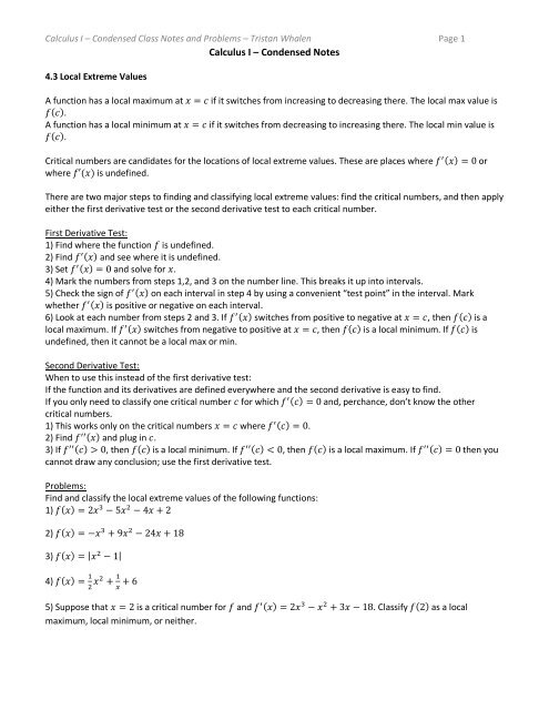
<strong>Calculus</strong> I <strong>–</strong> <strong>Condensed</strong> Class <strong>Notes</strong> and Problems <strong>–</strong> Tristan Whalen Page 1<br />
<strong>Calculus</strong> I <strong>–</strong> <strong>Condensed</strong> <strong>Notes</strong><br />
4.3 Local Extreme Values<br />
A function has a local maximum at if it switches from increasing to decreasing there. The local max value is<br />
( ).<br />
A function has a local minimum at if it switches from decreasing to increasing there. The local min value is<br />
( ).<br />
Critical numbers are candidates for the locations of local extreme values. These are places where ( ) or<br />
where ( ) is undefined.<br />
There are two major steps to finding and classifying local extreme values: find the critical numbers, and then apply<br />
either the first derivative test or the second derivative test to each critical number.<br />
First Derivative Test:<br />
1) Find where the function is undefined.<br />
2) Find ( ) and see where it is undefined.<br />
3) Set ( ) and solve for .<br />
4) Mark the numbers from steps 1,2, and 3 on the number line. This breaks it up into intervals.<br />
5) Check the sign of ( ) on each interval in step 4 by using a convenient “test point” in the interval. Mark<br />
whether ( ) is positive or negative on each interval.<br />
6) Look at each number from steps 2 and 3. If ( ) switches from positive to negative at , then ( ) is a<br />
local maximum. If ( ) switches from negative to positive at , then ( ) is a local minimum. If ( ) is<br />
undefined, then it cannot be a local max or min.<br />
Second Derivative Test:<br />
When to use this instead of the first derivative test:<br />
If the function and its derivatives are defined everywhere and the second derivative is easy to find.<br />
If you only need to classify one critical number for which ( ) and, perchance, don’t know the other<br />
critical numbers.<br />
1) This works only on the critical numbers where ( ) .<br />
2) Find ( ) and plug in .<br />
3) If ( ) , then ( ) is a local minimum. If ( ) , then ( ) is a local maximum. If ( ) then you<br />
cannot draw any conclusion; use the first derivative test.<br />
Problems:<br />
Find and classify the local extreme values of the following functions:<br />
1) ( )<br />
2) ( )<br />
3) ( ) | |<br />
4) ( )<br />
5) Suppose that is a critical number for and ( ) . Classify ( ) as a local<br />
maximum, local minimum, or neither.
<strong>Calculus</strong> I <strong>–</strong> <strong>Condensed</strong> Class <strong>Notes</strong> and Problems <strong>–</strong> Tristan Whalen Page 2<br />
4.4 Absolute Extreme Values<br />
An absolute maximum value of a function is a value the function takes (so, a number in the range of the function)<br />
that is bigger than or equal to any other value of the function.<br />
An absolute minimum value of a function is a value the function takes (so, a number in the range of the function)<br />
that is smaller than or equal to any other value of the function.<br />
Examples:<br />
( ) has no absolute maximum, and it has an absolute minimum of .<br />
( )<br />
( )<br />
has no absolute maximum and no absolute minimum.<br />
( ) has no absolute minimum, and it has an absolute maximum of<br />
If we look at a function on a closed interval [ ], then ( ) and ( ) may be either an endpoint minimum or an<br />
endpoint maximum. We figure out which using the first derivative. Use the steps of the first derivative test and<br />
include and on the ends of the intervals for checking in step 4.<br />
Examples:<br />
( ) on [ ] has an endpoint minimum of ( ) and an endpoint maximum of ( )<br />
( ) ( ) on [ ] has an endpoint maximum of ( ) and of ( )<br />
A continuous function is guaranteed to have both an absolute maximum and an absolute minimum on a closed<br />
interval [ ], so these are typical situations for problems involving absolute values.<br />
STUDY TIP: Most of the steps below are the same as the steps for local extreme values.<br />
Finding local, endpoint, and absolute extreme values of a continuous function on [ ]:<br />
1) Find ( )<br />
2) Set ( ) and solve for . Ignore any values that are not between and .<br />
3) Make a number line with on the left end, on the right end, and every number from step 2 in between. This<br />
breaks up the interval [ ] into some intervals to check (unless there are no numbers in step 2, and there is only<br />
one interval to check).<br />
4) Check the sign of ( ) on each interval in step 3 by using a convenient “test point” in the interval. Mark<br />
whether ( ) is positive or negative on each interval.<br />
[Steps 5 and 6 are wordy but easier to see on a picture]<br />
5) Classify the left endpoint. If ( ) is positive immediately to the right of , then ( ) is an endpoint minimum.<br />
If ( ) is negative immediately to the right of , then ( ) is an endpoint maximum.<br />
6) Classify the right endpoint. If ( ) is positive immediately to the left of , then ( ) is an endpoint maximum.<br />
If ( ) is negative immediately to the left of , then ( ) is an endpoint minimum.<br />
7) Look at each number from steps 2. If ( ) switches from positive to negative at , then ( ) is a local<br />
maximum. If ( ) switches from negative to positive at , then ( ) is a local minimum.<br />
8) Finally, if you haven’t already, plug in the numbers to get the function values at each number from step 2 and<br />
also get ( ) and ( ). The biggest number is the absolute maximum of on [ ]. The smallest number is the<br />
absolute minimum of on [ ].<br />
Problems:<br />
Find the critical numbers and classify the extreme values of the function on the interval:<br />
1) ( ) on [ ]:<br />
2) ( ) on [ ]
<strong>Calculus</strong> I <strong>–</strong> <strong>Condensed</strong> Class <strong>Notes</strong> and Problems <strong>–</strong> Tristan Whalen Page 3<br />
4.5 Max/Min Problems<br />
These are word problems for finding minimum or maximum values.<br />
1) What needs to be maximized or minimized? (the biggest volume, the smallest surface area, etc.)<br />
2) What are the parameters or restrictions? (A certain perimeter, a certain amount of material, etc.)<br />
3) Assign variables. Write the restriction in step 2 as an equation. Write the quantity in step 1 as an equation as<br />
well (could involve area or volume formula, for example).<br />
4) Using the restriction, get the quantity you’re trying to max/minimize in terms of one variable. Now it’s a<br />
function that we can the derivative of and apply methods from before.<br />
5) Take the derivative, find the critical number(s), among these find the location of the maximum or minimum.<br />
6) Depending on the question, write the final answer. This could be the critical number itself where the max/min<br />
occurs, or you may have to plug it in to the quantity in step 4.<br />
Problems:<br />
1) Find the minimum value of given that .<br />
2) A rectangle is drawn with its base on the -axis and its top two corners on the graph of What’s the<br />
largest possible area of such a rectangle?<br />
3) (a) If you have feet of fencing to enclose a rectangular yard against a building, what’s the largest possible area<br />
you could enclose?<br />
3) (b) If you need to enclose a rectangular yard of size square feet against a building, what’s the least amount of<br />
fencing you would need?<br />
4) What point on the graph of is closest to the point (<br />
5) If you need to make a rectangular box with square ends with a capacity of cubic feet, what’s the least amount<br />
of material you’d need?<br />
4.6 Concavity<br />
The second derivative tells us about the concavity of a function. Wherever ( ) , is concave up. Wherever<br />
( ) , is concave down.<br />
Note: Since ( ) is the derivative of ( ), we can figure out where is concave up by finding where ( ) is<br />
increasing. We can figure out where is concave down by finding where ( ) is decreasing.<br />
Analyzing Concavity:<br />
1) Make note of where is undefined.<br />
2) Find ( ) and make note of where ( ) is undefined.<br />
3) Set ( ) and solve for .<br />
4) Mark the numbers from steps 1,2, and 3 on a number line. This breaks it up into intervals you have to check.<br />
5) Pick a convenient “test point” from each interval in step 4 and plug it into ( ). All you need is whether ( )<br />
is positive or negative on each interval.<br />
6) If ( ) switches from positive to negative (or vice versa) at some point and ( ) is defined, then ( ( )) is<br />
a point of inflection.<br />
)?
<strong>Calculus</strong> I <strong>–</strong> <strong>Condensed</strong> Class <strong>Notes</strong> and Problems <strong>–</strong> Tristan Whalen Page 4<br />
Problems:<br />
Describe the concavity of the function and all points of inflection:<br />
1) ( )<br />
2) ( )<br />
3) ( )<br />
4) ( )<br />
4.7 Asymptotes, Vertical Tangents, and Cusps<br />
Vertical Asymptotes occur at points of infinite discontinuity. These are vertical lines with equation .<br />
Examples:<br />
1) ( )<br />
2) ( )<br />
has as a vertical asymptote<br />
has as a vertical asymptote and no others.<br />
Horizontal Asymptotes are horizontal lines at which the function’s graph “levels off”, that is, when one of the<br />
limits exists:<br />
( )<br />
These limits can be determined easily for rational functions, that is, a polynomial divided by a polynomial:<br />
( )<br />
( )<br />
( )<br />
If (the degree of the top and bottom are the same) then<br />
is the horizontal asymptote.<br />
( )<br />
If (the degree is smaller on top) then it is “bottom-heavy” and<br />
is the horizontal asymptote.<br />
If (the degree is bigger on top) then it is “top-heavy” and there is no horizontal asymptote.<br />
Vertical Tangents occur wherever the function has a “vertical tangent line.” That is, places where:<br />
( )<br />
Examples:<br />
( ) ( )<br />
has a vertical tangent at .<br />
( ) ( )<br />
has a vertical tangent at .
<strong>Calculus</strong> I <strong>–</strong> <strong>Condensed</strong> Class <strong>Notes</strong> and Problems <strong>–</strong> Tristan Whalen Page 5<br />
Vertical Cusps occur at sharp points in the graph of the function, wherever the derivative approaches from one<br />
direction but from the other.<br />
Examples:<br />
has a vertical cusp at .<br />
has a vertical cusp at .<br />
( ) ( )<br />
( ) ( )<br />
To find vertical tangents or cusps, begin by taking the derivative and if necessary simplify it (into one big fraction,<br />
for example). Usually you will look for where the derivative has division by 0, and then look at the power (the<br />
numerator of the exponent). Even powers cancel negative signs, so in this situation there probably is a vertical<br />
tangent. Odd powers do not cancel negative signs, so in this situation there is probably a vertical cusp. Note that<br />
vertical tangents/cusps automatically only happen where the derivative does not exist (is undefined).<br />
Problems:<br />
1) Find the horizontal and vertical asymptotes (if any):<br />
( )<br />
( )<br />
( )<br />
( )<br />
( )<br />
2) Find the vertical tangents and vertical cusps (if any):<br />
( ) ( )<br />
( ) ( )<br />
( ) ( )<br />
( ) ( )<br />
( ) ( )
<strong>Calculus</strong> I <strong>–</strong> <strong>Condensed</strong> Class <strong>Notes</strong> and Problems <strong>–</strong> Tristan Whalen Page 6<br />
4.8 Curve Sketching<br />
This combines the previous sections. Here is what is usually involved:<br />
1) Domain of ( ) (note points where is not defined)<br />
2) Vertical and horizontal asymptotes (section 4.7)<br />
3) Use the first derivative to determine where is increasing or decreasing (section 4.2-4.3)<br />
4) Use the second derivative to determine where is concave up or down (section 4.6)<br />
6) Plot the asymptotes and the points of interest (places increasing/decreasing changes, places concavity changes,<br />
etc). This includes getting the function value at the point so you know the -value to plot!<br />
7) Sketch the graph by connecting the dots or asymptotes from step 6 with the appropriate shape of curve<br />
(increasing and concave up; increasing and concave down; decreasing and concave up; decreasing and concave<br />
down).<br />
Notice that if you need local max or min values, you get these automatically with step 4 (the first derivative) and if<br />
you need points of inflection, you get these automatically with step 5 (the second derivative)<br />
You may also want to find the -intercepts (get ( )) or -intercepts (solve ( ) ). If applicable, determine<br />
symmetry and periodicity (this will be clear, such as if you have a trig function). But focus on the steps above.<br />
Problems:<br />
1) Sketch a graph of the following functions:<br />
( )<br />
( )<br />
( )<br />
2) Here is a function and its first and second derivatives:<br />
Sketch a graph of .<br />
( )<br />
( )<br />
( )<br />
( )<br />
( )<br />
( )<br />
3) Which of the following is true about the graph of the function ( ) ?<br />
A) has a point of inflection at the point ( )<br />
B) is decreasing on the interval (<br />
C) has a local minimum at the point ( )<br />
D) has a local maximum at the point ( )<br />
E) is increasing on the interval (<br />
)<br />
)
<strong>Calculus</strong> I <strong>–</strong> <strong>Condensed</strong> Class <strong>Notes</strong> and Problems <strong>–</strong> Tristan Whalen Page 7<br />
5.2 The Area Problem and the Integral<br />
When we want the area of a region that is not rectangular, we can approximate it using rectangles. If that region<br />
is between a function’s graph and the -axis from to , these are the methods to approximate that area.<br />
Chop up the interval [ ] into a “partition” . Each piece/slice of this partition is the base of a rectangle.<br />
Put the top of the rectangle on each slice on the graph of the function using:<br />
Left Endpoints: just put the top-left corner of each rectangle on the graph of the function<br />
Right Endpoints: just put the top-right corner of each rectangle on the graph of the function<br />
Midpoints: put the middle of the rectangle on the graph of the function<br />
<br />
Upper Sum: each rectangle’s height is the largest function value over that slice<br />
Lower Sum: each rectangle’s height is the smallest function value over that slice<br />
Riemann Sum: each rectangle’s height is an arbitrary value of the function over that slice<br />
All of this approximating is really in hopes of finding the exact, true area of the region, represented by the integral<br />
symbol:<br />
∫ ( )<br />
This represents the number which is the area of the region between the graph of , the -axis, from to . Since<br />
this is just a number, the variable in the integral is called a “dummy-variable.”<br />
Problems:<br />
1) Find the upper sum for ( ) with the partition {<br />
2) Find the lower sum for ( ) with the partition {<br />
}<br />
}
<strong>Calculus</strong> I <strong>–</strong> <strong>Condensed</strong> Class <strong>Notes</strong> and Problems <strong>–</strong> Tristan Whalen Page 8<br />
3) (a) Using the partition { }, draw the rectangles involved in the upper sum ( ) on<br />
the graph of below. Then find the upper sum.<br />
3) (b) Using the partition { }, draw the rectangles involved in the lower sum ( ) on the<br />
graph of below. Then find the lower sum.<br />
4) What is the actual area between the graph of and the -axis from to , where is graphed above for<br />
problem 3? That is, find<br />
∫ ( )
<strong>Calculus</strong> I <strong>–</strong> <strong>Condensed</strong> Class <strong>Notes</strong> and Problems <strong>–</strong> Tristan Whalen Page 9<br />
5.3 The integral as a function<br />
Given a function we can set<br />
where the input is the upper limit .<br />
We have that if is continuous and , then<br />
If is continuous,<br />
Another way to write that is:<br />
( ) ∫ ( )<br />
∫ ( ) ∫ ( ) ∫ ( )<br />
( ) ( )<br />
(∫ ( )<br />
) ( )<br />
If we compose with another function and want the derivative, then by the Chain Rule:<br />
Putting all this together,<br />
Examples:<br />
(∫<br />
Problems:<br />
1) If you know the following<br />
evaluate the following integrals:<br />
( )<br />
(∫ ( )<br />
( )<br />
( )<br />
(∫ ( )<br />
(∫ ( )<br />
(∫<br />
) ( ( )) ( )<br />
) ( ( )) ( ) ( ( )) ( )<br />
) ( ) ( ) ( )<br />
)<br />
) ( ( ) ( ) )( ) ( )( )<br />
∫ ( )<br />
∫ ( )<br />
∫ ( )<br />
∫ ( )<br />
∫ ( )<br />
∫ ( )<br />
∫ ( )
<strong>Calculus</strong> I <strong>–</strong> <strong>Condensed</strong> Class <strong>Notes</strong> and Problems <strong>–</strong> Tristan Whalen Page 10<br />
2) Find these derivatives:<br />
(∫ √<br />
(∫ ( )<br />
3) Solve for the function . Then find ( )<br />
4) If<br />
)<br />
)<br />
( ) ∫<br />
find (a) ( ), (b) ( ), (c) the critical numbers of ( ).<br />
5.4 The Fundamental Theorem of <strong>Calculus</strong><br />
∫<br />
( )<br />
(∫ ( )<br />
)<br />
(∫ ( )<br />
√<br />
An antiderivative for is a function where ( ) ( ). The only difference between any two antiderivatives<br />
for a given function is adding a constant.<br />
If ( ) is continuous, then<br />
∫ ( )<br />
is an antiderivative of ( ) (where the lower limit is a constant), and if ( ) is any antiderivative of , then<br />
∫ ( ) ( ) ( )<br />
We can find many antiderivatives by “undoing” derivatives we already know.<br />
Function Antiderivative<br />
( ) ( )<br />
( ) ( )<br />
e ( ) ta ( )<br />
e ( ) ta ( ) e ( )<br />
( ) t( ) ( )<br />
( ) t( )<br />
)
<strong>Calculus</strong> I <strong>–</strong> <strong>Condensed</strong> Class <strong>Notes</strong> and Problems <strong>–</strong> Tristan Whalen Page 11<br />
Evaluating a definite integral<br />
1) Simplify the integrand as much as possible<br />
2) Compare the integrand with the antiderivative chart<br />
3) Using the chart and integration techniques (to be explored in section 5.7 and <strong>Calculus</strong> II) find the antiderivative<br />
of the integrand.<br />
4) Plug in the limits and subtract in the correct order: [antiderivative evaluated at upper limit] minus<br />
[antiderivative evaluated at lower limit]<br />
Examples:<br />
∫<br />
√<br />
5.5 Area Problems<br />
∫ √<br />
[<br />
( )<br />
∫<br />
|<br />
( )<br />
∫ e ( ) ta ( )|<br />
[<br />
( ) ] [<br />
( )<br />
]<br />
[<br />
( )<br />
ta (<br />
) ta (<br />
]<br />
( ) ] [<br />
( )<br />
) √<br />
( ) ] [<br />
( )<br />
( ) ]<br />
When the function is positive over the interval, then the integral gives<br />
the area we want:<br />
When the function is negative over the interval, then the integral gives us the area of the region but negative.<br />
When we want the area of a region bounded by two functions, we will determine where each function is on top<br />
or on bottom of the region, and subtract.
<strong>Calculus</strong> I <strong>–</strong> <strong>Condensed</strong> Class <strong>Notes</strong> and Problems <strong>–</strong> Tristan Whalen Page 12<br />
To get the area of the region below ( ) (so is on top), above ( ) (so is on bottom), and between and ,<br />
we use:<br />
∫ ( ) ∫ ( )<br />
Integrate the TOP function minus the BOTTOM function.<br />
∫ ( ( ) ( ))<br />
If we have two functions and they criss-cross, we just use more than one integral. If we have just one function and<br />
the -axis, treat as the second function. Then this method of “top minus bottom” will always give us the<br />
area.<br />
Finding Area of Region bounded by two functions<br />
1) Find the intersections of the two functions by setting them equal and solving for<br />
(even if one of the functions is , the -axis).<br />
2) If you have two points, you will need one integral. If you have three points, you will need two integrals. And so<br />
on. Include in the points any boundaries given in the problem (a vertical line )<br />
3) In between each pair of points from step 1, figure out which function is on top with a test value in between.<br />
4) Set up each integral. The limits are, from left to right, each pair of points. The integrand is the top function<br />
minus the bottom function for each pair of points.<br />
5) Evaluate the integrals using the Fundamental Theorem of <strong>Calculus</strong>, then add them up.<br />
Example:<br />
Find the area of the region between the graph and the -axis.<br />
1) Set equal to . Then we have , so ( ) , so we get .<br />
2) We’ll need two integrals since we have 3 points.<br />
3) Work from left to right. In between the first pair and , we check using<br />
(<br />
)<br />
so is on top.<br />
In between the second pair and , we check using<br />
axis) is on top.<br />
Next page…<br />
that (<br />
)<br />
(<br />
)<br />
to see that (<br />
)<br />
so (the -
<strong>Calculus</strong> I <strong>–</strong> <strong>Condensed</strong> Class <strong>Notes</strong> and Problems <strong>–</strong> Tristan Whalen Page 13<br />
4) For the first pair of points, we had to and on top, so:<br />
∫ ( ) ( )<br />
For the second pair of points, we had to and -axis on top, so:<br />
5)<br />
∫ ( ) ( )<br />
And the area is<br />
Problems:<br />
∫ ( ) ( )<br />
∫ ( ) [<br />
∫ [<br />
∫ ( ) ( )<br />
]<br />
[<br />
]<br />
)<br />
] [(<br />
[<br />
] [<br />
( )<br />
1) Sketch and find the area of the region bounded by the graphs of and .<br />
2) Sketch and find the area of the region bounded by the graphs of ( ) and ( ) .<br />
3) Sketch and find the area of the region bounded by ( ) ( ) and the -axis between and .<br />
4) Sketch and find the area of the region bounded by ( ) ( ) and ( ) ( ) between and<br />
.<br />
5) Sketch and find the area of the region bounded by ( ) ( ), ( ) ( ), AND the -axis between<br />
and .<br />
6) Sketch and find the area of the region bounded by ( ) and ( ) .<br />
Still remaining are sections 5.6 through 5.9.<br />
]<br />
]<br />
(<br />
)
<strong>Calculus</strong> I <strong>–</strong> <strong>Condensed</strong> Class <strong>Notes</strong> and Problems <strong>–</strong> Tristan Whalen Page 14<br />
Some practice problems:<br />
Section 5.6<br />
Section 5.7<br />
∫( )<br />
∫ ( )<br />
∫ √<br />
( )( √ )<br />
∫<br />
∫ ( )<br />
∫ √<br />
∫ ( ) ( )<br />
∫ ( )


