Parabolic cylinder functions - Read

Parabolic cylinder functions
E. Cojocaru
Department of Theoretical Physics, Horia Hulubei
National Institute of Physics and Nuclear Engineering,
Magurele-Bucharest P.O.Box MG-6, 077125 Romania ∗
Routines for computation of Weber’s parabolic cylinder functions and their deriva-
tives are provided for both moderate and great values of the argument. Standard,
real solutions are considered. Tables of values are included.
∗ Electronic address: ecojocaru@theory.nipne.ro

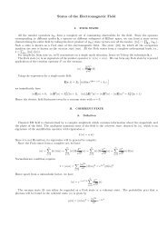
I. INTRODUCTION
The parabolic cylinder functions were introduced by Weber [1] in 1869. Standard solu-
tions to Weber’s equation were given by Miller [2] in 1952. These relations are also provided
by Abramowitz and Stegun [3]. There are two standard forms of the Weber’s equation,
d2y − (1
dx2 4 x2 + a)y = 0, (1)
d2y + (1
dx2 4 x2 − a)y = 0. (2)
Equation (2) is obtained from (1) with changes a by −ia and x by xe iπ/4 . Thus, if y(a, x)
is a solution of (1), then (2) has solutions: y(−ia, xe iπ/4 ), y(−ia, −xe iπ/4 ), y(ia, −xe −iπ/4 ),
and y(ia, xe −iπ/4 ). In the following we consider only real solutions of real equations.
II. SOLUTIONS OF EQUATION (1)
A. Standard solutions
There are two standard solutions of Eq. (1), U(a, x) and V (a, x), both of them expressed
in terms of Whittaker’s function D 1
−a− ,
2
U(a, x) = D 1
−a− , (3)
2
V (a, x) = 1
π Γ(1 + a)[sin(πa)U(a, x) + U(a, −x)]. (4)
2
In a more symmetrical notation, these solutions are
where
U(a, x) = D −a− 1
2
V (a, x) =
Y1 =
1 y1Γ( 4
√ a 1
+ π2 2 4
= Y1cosβ − Y2sinβ, (5)
1
Γ( 1
2 − a)(Y1sinβ + Y2cosβ), (6)
β = π( a
2
a − 2 )
, Y2 =
1
+ ), (7)
4
3 y2Γ( 4
√ a 1
− π2 2 4
2
a − 2 )
, (8)
y1 = 1 + a x2
2! + (a2 + 1
2 )x4
4! + (a3 + 7a
2 )x6
6! + (a4 + 11a 2 + 15
4 )x8 + . . . , (9)
8!

y2 = x + a x3
3! + (a2 + 3
2 )x5
5! + (a3 + 13a
2 )x7
7! + (a4 + 17a 2 + 63
4 )x9 + . . . , (10)
9!
in which the coefficients An of xn
n!
Similarly to Eq. (4), there is relation
At x = 0,
U(a, x) =
obey the recurrence relation
An+2 = aAn + 1
4 n(n − 1)An−2. (11)
π
Γ(a + 1
2 )cos2 [V (a, −x) − sin(πa)V (a, x)]. (12)
(πa)
U(a, 0) =
U ′ (a, 0) = −
V (a, 0) =
V ′ (a, 0) =
√ π
2 a 1
+ 2 4 Γ( a
2
√ π
+ 3
4 ),
2 a 1
− 2 4 Γ( a 1 + 2 4 ),
a 1
+ 2 2 4 sinπ( 3 a − 4
Γ( 3
4
− a
2 )
a 3
+ 2 2 4 sinπ( 1
4
Γ( 1
4
2 )
,
3
(13)
a − 2 )
a − 2 )
, (14)
B. Recurrence relations for U(a, x) and V (a, x)
Standard solutions U(a, x) and V (a, x) obey the recurrence relations
xU(a, x) − U(a − 1, x) + (a + 1
)U(a + 1, x) = 0,
2
U ′ (a, x) − 1
xU(a, x) + U(a − 1, x) = 0, (15)
2
xV (a, x) − V (a + 1, x) + (a − 1
)V (a − 1, x) = 0,
2
V ′ (a, x) − 1
1
xV (a, x) − (a − )V (a − 1, x) = 0. (16)
2 2
C. Relations at large values of argument x
At large values of argument x, when x ≫ |a|, there are relations
1 x2
−a− −
U(a, x) ∼ x 2 e 4 [1 −
V (a, x) ∼
2 1
xa− 2 e
π x2
4 [1 +
1 3
(a + )(a + 2 2 )
2x2 + (a + 1
1 3
(a − )(a − 2 2 )
2x2 + (a − 1
2
2
)(a + 3
2
)(a − 3
2
5 7
)(a + )(a + 2 2 )
2 · 4x 4 − . . . ], (17)
5 7
)(a − )(a − 2 2 )
2 · 4x 4 + . . . ]. (18)

III. SOLUTIONS OF EQUATION 2
A. Standard solution
The standard solution W (a, x) of Eq. (2) is
where
3
−
W (a, ±x) = 2 4 (
G1
y1 ∓
G3
4
2G3
y2), (19)
G1 = |Γ(ia + 1
4 )|, G3 = |Γ(ia + 3
)|,
4
(20)
y1 = 1 + a x2
2! + (a2 − 1
2 )x4
4! + (a3 − 7a
2 )x6
6! + (a4 − 11a 2 + 15
4 )x8 + . . . ,
8!
(21)
y2 = x + a x3
3! + (a2 − 3
2 )x5
5! + (a3 − 13a
2 )x7
7! + (a4 − 17a 2 + 63
4 )x9 + . . . ,
9!
(22)
in which the coefficients An of xn
n!
G1
obey the recurrence relation
An+2 = aAn − 1
4 n(n − 1)An−2. (23)
Relations for gamma function of complex argument are given in Appendix A. At x = 0,
3
− G1
W (a, 0) = 2 4
G3
W ′ 1
−
(a, 0) = −2 4
G3
B. Relations at large values of argument x
,
. (24)
G1
At large values of the argument x, when x ≫ |a|, there are relations
2k
W (a, x) =
x [s1(a, x) cos γ − s2(a, x) sin γ],
2
W (a, −x) =
kx [s1(a, x) sin γ + s2(a, x) cos γ], (25)
where
with
k = √ 1 + e 2πa − e πa , k −1 = √ 1 + e 2πa + e πa , (26)
γ = x2
4
− a ln x + π
4
φ
+ , (27)
2
φ = arg Γ(ia + 1
), (28)
2

with
s1(a, x) ∼ 1 + v2 u4
−
1!2x2 2!22 v6
−
x4 3!23 u8
+
x6 4!24 + . . . , (29)
x8 s2(a, x) ∼ − u2 v4
−
1!2x2 2!22 u6
+
x4 3!23 v8
+
x6 4!24 − . . . , (30)
x8 um + ivm =
At a = 0 there are relations
1
Γ(m + ia + 2 )
, m = 2, 4, 6 . . . (31)
Γ(ia + 1
2 )
C. Analytic relations at a = 0
W (0, ±x) = 2
dW (0, ±x)
dx
5
− 4
√
πx
J − 1
4
9
−
= −2 4 x √
πx
2 x
J 3
4
where Jν(z) is the Bessel function of the first kind.
4
2 x
4
∓ J 1
4
x 2
± J − 3
4
4
5
, (32)
x 2
4
, (33)
IV. IMPLEMENTATION OF PARABOLIC CYLINDER FUNCTIONS IN
MATLAB
Routines provided for computation of parabolic cylinder functions are shortly described
in Table I. For moderate values of argument x and parameter a, standard parabolic cylin-
der functions U(a, x) and V (a, x) are computed with routines “pu” and “pv”, respectively,
whereas W (a, x) is computed with routine “pw”. Differentiation with respect to argument
x is computed with routines “dpu”, “dpv”, and “dpw”. For large values of argument x,
when |x| ≫ |a|, functions U(a, x), V (a, x), and W (a, x) are computed with routines “pulx”,
“pvlx”, and “pwlx”, and their derivatives with routines “dpulx”, “dpvlx”, and “dpwlx”,
respectively. Routine “cgamma” computes the gamma function of complex argument; using
the function code kf, it computes either the logarithm of gamma function (when kf = 0)
or gamma function (when kf = 1). Values of parabolic cylinder functions obtained by using
these routines are shown in Tables II–VII.

APPENDIX A: RELATIONS FOR GAMMA FUNCTION OF COMPLEX
ARGUMENT
If |z| ≫ 1 and | arg z| ≤ π − ɛ with ɛ > 0, there is relation
ln Γ(z) ∼ (z − 1
1
) ln z − z + ln 2π +
2 2
where B2n are the Bernoulli’s numbers,
Specific values,
Other useful relations,
k−1 2 · (2k)!
B2k = (−1)
(2π) 2k
∞
n=1
n=1
B2 = 1/6 B12 = −691/2730
B4 = −1/30 B14 = 7/6
6
∞ B2n 1
, (A1)
2n(2n − 1) z2n−1 1
, k = 1, 2, . . . (A2)
n2k B6 = 1/42 B16 = −3617/510 (A3)
B8 = −1/30 B18 = 43867/798
B10 = 5/66 B20 = −174611/330
Γ(z + n) = z(z + 1) · · · (z + n − 1)Γ(z),
Γ(z)Γ(−z) = −π
z sin πz
(A4)
[1] H. F. Weber “Ueber die Integration der partiellen Differential-gleichung: ∂ 2 u/∂x 2 + ∂ 2 u/∂y 2 +
k 2 u = 0,” Math. Ann. 1, 1–36 (1869).
[2] J. C. P. Miller “On the choice of standard solutions to Weber’s equation,” Proc. Cambridge
Philos. Soc. 48, 428–435 (1952).
[3] M. Abramowitz and I. Stegun Handbook of Mathematical Functions (New York, 1964).

TABLE I: Routines for parabolic cylinder functions
Name of routine Routine call What the routine computes
cgamma [gr, gi]=cgamma(x, y, kf) Γ(z) with complex argument z (when kf = 1) or ln Γ(z),
(when kf = 0); x and y are the real and imaginary parts of z
gr and gi are the real and imaginary parts of ln Γ(z) or Γ(z)
[Eqs. (A1–A4)].
pu u=pu(a, x) Parabolic cylinder function U(a, x) for moderate values of
parameter a and argument x [Eqs. (3–12)].
dpu du=dpu(a, x) Derivative with respect to x of parabolic cylinder function
U(a, x) for moderate values of parameter a and argument x
pv v=pv(a, x) Parabolic cylinder function V (a, x) for moderate values of
parameter a and argument x [Eqs. (3–12)].
dpv dv=dpv(a, x) Derivative with respect to x of parabolic cylinder function
V (a, x) for moderate values of parameter a and argument x
pw w=pw(a, x) Parabolic cylinder function W (a, x) for moderate values of
parameter a and argument x [Eqs. (19–23)].
dpw dw=dpw(a, x) Derivative with respect to x of parabolic cylinder function
W (a, x) for moderate values of parameter a and argument x
pulx u=pulx(a, x) Parabolic cylinder function U(a, x) for large values of parameter
x (|x| ≫ |a|) and moderate values of parameter a [Eq. (17)].
dpulx du=dpulx(a, x) Derivative with respect to x of parabolic cylinder function
U(a, x) for large values of parameter x (|x| ≫ |a|) and moderate
values of parameter a.
pvlx v=pvlx(a, x) Parabolic cylinder function V (a, x) for large values of parameter
x (|x| ≫ |a|) and moderate values of parameter a [Eq. (18)].
dpvlx dv=dpvlx(a, x) Derivative with respect to x of parabolic cylinder function
V (a, x) for large values of parameter x (|x| ≫ |a|) and moderate
values of parameter a.
pwlx w=pwlx(a, x) Parabolic cylinder function W (a, x) for large values of parameter
x (|x| ≫ |a|) and moderate values of parameter a [Eqs. (25–31)].
dpwlx dw=dpwlx(a, x) Derivative with respect to x of parabolic cylinder function
W (a, x) for large values of parameter x (|x| ≫ |a|) and moderate
values of parameter a.
7

TABLE II: Values of U(a, x) with a = −5, −3.5, −1, 1, 3.5, 5 and x = 0, 1, 3, 5
x\a -5.0 -3.5 -1.0
0.0 3.052183664350372 -0.000000000000000 0.581368317019118
1.0 0.579926011661105 -1.557601566142810 0.842203244069839
3.0 3.202129097812791 1.897186042113549 0.184881790005045
5.0 1.879976816310843 0.212349954984646 0.004337473181400
x\a 1.0 3.5 5.0
0.0 1.162736634038237 0.333333333333333 0.103354367470066
1.0 0.378262434740955 0.048971230815929 0.010659966828235
3.0 0.017224293634316 0.000610423938072 0.000070950238455
5.0 0.000161381143270 0.000002208878109 0.000000155227075
TABLE III: Values of U(a, −x) with a = −5, −3.5, −1, 1, 3.5, 5 and x = 0, 1, 3, 5
x\a -5.0 -3.5 -1.0
0.0 3.052183664350372 -0.000000000000000 0.581368317019118
1.0 -4.332232266251285 1.557601566142810 -0.195001018223362
3.0 3.802753160685226 -1.897186042113549 -1.767855400724101
5.0 -9.615606269532364 -0.212349954984649 -35.754085404247576
x\a 1.0 3.5 5.0
0.0 1.16273663404 0.33333333333 0.10335436747
1.0 3.27078479478 2.19468750736 0.97838806074
3.0 45.73101176423 142.69397188181 125.30190015651
5.0 3259.12460949910 30297.53050402874 45998.28922772748
8

TABLE IV: Values of V (a, x) with a = −5, −3.5, −1, 1, 3.5, 5 and x = 0, 1, 3, 5
x\a -5.0 -3.5 -1.0
0.0 -0.058311457540778 0.265961520267622 -0.656003897333753
1.0 0.082766571619165 -0.076762147625440 0.220035086525655
3.0 -0.072650962016911 0.097154672861824 1.994811204614366
5.0 0.183704546768818 1.173350875864019 40.344165108706711
x\a 1.0 3.5 5.0
0.0 0.3280019487 0 1.7220102305
1.0 0.9226713556 4.0980162226 16.3011422859
3.0 12.9004802412 272.5242458690 2087.6829809173
5.0 919.3820780818 57864.0209141053 766387.7838412275
TABLE V: Values of V (a, −x) with a = −5, −3.5, −1, 1, 3.5, 5 and x = 0, 1, 3, 5
x\a -5.0 -3.5 -1.0
0.0 -0.058311457540778 0.265961520267622 -0.656003897333753
1.0 -0.011079389291262 -0.076762147625440 -0.950324595068664
3.0 -0.061176139925034 0.097154672861824 -0.208616760217021
5.0 -0.035916642101972 1.173350875864019 -0.004894314375732
x\a 1.0 3.5 5.0
0.0 0.32800194867 0 1.72201023050
1.0 0.10670586276 -4.09801622261 0.17760809131
3.0 0.00485888353 -272.52424586904 0.00118211779
5.0 0.00004552478 -57864.02091410524 0.00000258678
9

TABLE VI: Values of W (a, x) with a = −5, −3, −1, 1, 3, 5 and x = 0, 1, 3, 5
x\a -5.0 -3.0 -1.0
0.0 0.473478576486605 0.539330386270653 0.731481090245431
1.0 -0.657520526362908 -0.611126375982879 -0.184115556183355
3.0 -0.062604004232077 0.636305300554784 -0.053352644054153
5.0 0.089361847055232 0.437066960213013 -0.570254174032845
x\a 1.0 3.0 5.0
0.0 0.731481090245431 0.539330386270653 0.473478576486605
1.0 0.315937643962764 0.101682226485666 0.052572013487910
3.0 0.016773032899024 0.009166528652640 0.001223742332881
5.0 0.022807516888135 -0.003844865237560 0.000115773464320
TABLE VII: Values of W (a, −x) with a = −5, −3, −1, 1, 3, 5 and x = 0, 1, 3, 5
x\a -5.0 -3.0 -1.0
0.0 0.473478576486605 0.539330386270653 0.731481090245431
1.0 0.070610950611453 0.428801301530536 0.950916920458344
3.0 0.606270877302830 0.177268761402591 -0.757374330077355
5.0 0.538608396875686 -0.370945283780393 0.180907184885679
x\a 1.0 3.0 5.0
0.0 0.731481090245 0.539330386271 0.473478576487
1.0 1.903689596383 3.001251077335 4.378212848013
3.0 6.183176599808 57.210355295947 253.398744868662
5.0 -4.359927574948 66.590129609337 2852.835947866653
10