Hull-Appendage Interaction of a Sailing Yacht, Investigated with ...
Hull-Appendage Interaction of a Sailing Yacht, Investigated with ...
Hull-Appendage Interaction of a Sailing Yacht, Investigated with ...

Create successful ePaper yourself
Turn your PDF publications into a flip-book with our unique Google optimized e-Paper software.
<strong>Hull</strong>-<strong>Appendage</strong> <strong>Interaction</strong> <strong>of</strong> a <strong>Sailing</strong> <strong>Yacht</strong>, <strong>Investigated</strong> <strong>with</strong> Wave-Cut Techniques<br />
Jonathan R. Binns, Australian Maritime Engineering Cooperative Research Centre (AMECRC)<br />
Kim Klaka, Australian Maritime Engineering Cooperative Research Centre (AMECRC)<br />
Andrew Dovell, Iain Murray & Associates Pty Ltd<br />
ABSTRACT<br />
The research explained in this paper was carried<br />
out to investigate the effects <strong>of</strong> hull-appendage<br />
interaction on the resistance <strong>of</strong> a sailing yacht, and the<br />
effects these changes have on the velocity prediction<br />
for a sailing yacht. To accomplish this aim a series <strong>of</strong><br />
wave-cut experiments was carried out and analysed<br />
using a modified procedure. The processed results<br />
have then been incorporated into an existing velocity<br />
prediction program. For the purposes <strong>of</strong> this research<br />
two variables were investigated for the Australian<br />
Maritime Engineering Cooperative Research Centre<br />
(AMECRC) parent model 004, a model derived from<br />
the Delft IMS series <strong>of</strong> yachts.<br />
Wave-cut procedures inevitably raise questions<br />
about scaling procedures for full scale extrapolation as<br />
the inviscid wave-pattern resistance is calculated to be<br />
less than the residuary or wave resistance. These<br />
questions have been dealt <strong>with</strong> by an approximate<br />
method, briefly explained in this paper.<br />
NOTATION<br />
A Wetted surface area <strong>of</strong> model (m 2 )<br />
ARe Effective aspect ratio <strong>of</strong> lifting surface<br />
ARg Geometric aspect ratio<br />
Cdi Induced drag coefficient<br />
Cf Skin friction resistance coefficient<br />
Cl Lift coefficient<br />
Ct Total resistance coefficient<br />
Cw Assumed wave resistance or residuary<br />
resistance coefficient<br />
Cwp Wave-pattern resistance coefficient<br />
Di Induced drag due to three-dimensional lift<br />
production (N)<br />
Fn Froude number<br />
GPR General Purpose Rating (seconds per<br />
nautical mile)<br />
IMS International Measurement System<br />
k Form factor<br />
kΔ Form factor calculated from wave-pattern<br />
results, can vary <strong>with</strong> yacht speed<br />
L Lift (N)<br />
LR Linear Random<br />
Rf Skin friction resistance (N)<br />
Rn Reynolds number<br />
Rt Total resistance (N)<br />
Rv Total viscous resistance (N)<br />
Rw Assumed wave resistance or residuary<br />
resistance (N)<br />
Rwp Wave-pattern resistance (N)<br />
s Span <strong>of</strong> lifting surface (m)<br />
S Pr<strong>of</strong>ile area <strong>of</strong> lifting surface (m2 )<br />
Vs <strong>Yacht</strong> full scale predicted velocity (knots)<br />
VPP Velocity Prediction Program<br />
x Longitudinal dimension, aft positive<br />
y Transverse dimension, starboard positive<br />
z Vertical dimension, against gravity positive<br />
ρ Fluid density (kg/m 3 )<br />
ψ Yaw angle <strong>of</strong> yacht (degrees)<br />
ζ Wave height (m)<br />
INTRODUCTION<br />
The primary objective <strong>of</strong> the research has been to<br />
provide design information as to the effect <strong>of</strong> sailing<br />
yacht hull and appendage characteristics on the<br />
resistance <strong>of</strong> the yacht. It has been observed in yacht<br />
model tests that varying the appendages on a sailing<br />
hull appears to have the effect <strong>of</strong> changing the wavepattern<br />
around the yacht (for example see Rosen et al,<br />
1993). Therefore the wave-pattern was analysed by<br />
conducting a wave-cut program.<br />
The variables investigated were the keel rudder<br />
separation and the rudder angle. To investigate the<br />
overall effects <strong>of</strong> the appendages the model was also
tested <strong>with</strong> no appendages, <strong>with</strong> keel only and <strong>with</strong><br />
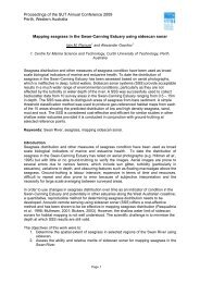
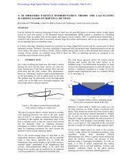
rudder only. Fig. 1 shows the six pr<strong>of</strong>iles <strong>of</strong> the<br />
models that were tested. It was found that the best<br />
performance prediction was obtained by locating the<br />
rudder as far aft as possible, <strong>with</strong> the smallest rudder<br />
angle possible. However, the steps taken in this<br />
research required some assumptions, which should<br />
guide the applications <strong>of</strong> this basic design principle<br />
(see Binns, 1996).<br />
Fig. 2 Model configurations tested<br />
By using wave-cut techniques it is possible to<br />
shed some light on the subject <strong>of</strong> scaling the results<br />
from the model to the prototype yachts. It has been<br />
concluded from this research that using a standard<br />
resistance scaling scheme the wave-pattern resistance<br />
is probably being overestimated, resulting in a 12%<br />
over prediction <strong>of</strong> the total resistance.<br />
The tank tests required for this research were<br />
carried out in the AMECRC towing tank based at the<br />
Australian Maritime College (AMC), Launceston,<br />
Tasmania. The tank has a rectangular cross section<br />
<strong>with</strong> a length <strong>of</strong> 60 m, width <strong>of</strong> 3.5 m and depth <strong>of</strong><br />
1.5 m.<br />
DIVISION OF RESISTANCE<br />
Basic Principles<br />
In order to analyse the resistance <strong>of</strong> a sailing<br />
yacht it is extremely useful to divide the total<br />
resistance into components. This is because the total<br />
resistance is due to fairly distinct phenomena and so<br />
different assumptions may be made for each<br />
component allowing for different prediction methods<br />
to be employed. Furthermore, the division <strong>of</strong><br />
resistance becomes critical when work is to be carried<br />
out at model scale and extrapolated to full scale.<br />
The resistance <strong>of</strong> a sailing yacht may be divided<br />
into three broad groups. The first group is that<br />
associated <strong>with</strong> gravity forces, the second that<br />
concerned <strong>with</strong> viscous forces and the third that due to<br />
the generation <strong>of</strong> lift on a three-dimensional body.<br />
The first group can be described by the wave surface<br />
energy around the yacht. The second and third groups<br />
can be observed and evaluated by measurements <strong>of</strong> the<br />
detailed sub-surface velocity field around the hull.<br />
Then these three components <strong>of</strong> resistance may be<br />
added to give the total resistance, easily measured at<br />
model scale as the force required to tow the vessel.<br />
A hierarchy <strong>of</strong> yacht resistance could be<br />
visualised as follows
Froude s caled res is tance g ro ups<br />
Fig. 3 Resistance hierarchy diagram.<br />
In this diagram wave-breaking resistance is seen<br />
to contribute to two resistance components. Also on<br />
the diagram groupings <strong>of</strong> resistance components have<br />
been shown for Reynolds and Froude scaling portions.<br />
The dashed lines show where traditional scaling<br />
methods divide the total resistance, and the solid lines<br />
show where wave-cut guided scaling methods divide<br />
the resistance. This shall be discussed in the<br />
following sections.<br />
Mainly due to the thin nature <strong>of</strong> most ships, the<br />
resistance due to viscous effects can be fairly well<br />
predicted by approximating the vessel to a flat plate.<br />
The third resistance group can be accurately predicted<br />
by potential flow theory at small angles <strong>of</strong> attack. By<br />
using these assumptions the wave resistance can be<br />
measured by subtracting the calculated viscous<br />
resistance from the total resistance. Generally this<br />
procedure is sufficient when separation <strong>of</strong> the flow<br />
around the vessel is small.<br />
In order to create side forces sailing yachts<br />
usually need to advance through the water <strong>with</strong> an<br />
angle <strong>of</strong> yaw. The side force can then be created by a<br />
symmetric lifting surface, for example a keel. The<br />
angle <strong>of</strong> yaw also creates a lot more separation around<br />
the hull and so increases the viscous resistance. This<br />
increase cannot be described by the use <strong>of</strong> a simple<br />
skin friction coefficient. Therefore in order to<br />
separate the resistance due to waves and the viscous<br />
Reyn olds s caled res is tance g ro ups<br />
resistance it is necessary to measure one or the other.<br />
If the relationship between wave height and wave<br />
energy is known, the wave-pattern resistance can be<br />
determined by measuring the wave-pattern around the<br />
yacht (Eggers et al, 1967); this is the basis <strong>of</strong> the<br />
research described here.<br />
Scaling <strong>of</strong> Resistance Components<br />
The laws <strong>of</strong> similitude have been well<br />
documented in the past and so will not be dealt <strong>with</strong><br />
here (see for example Harvald, 1983, pp 39-42),<br />
suffice to say that viscous resistance requires Reynolds<br />
scaling whereas resistance due to gravitational forces<br />
requires Froude scaling.<br />
A traditional approach to the problem <strong>of</strong> scaling<br />
model resistance which seems to be fairly widely used<br />
is that first described by Hughes and later modified by<br />
Prohaska (see Hughes, 1966). This method involves<br />
using a skin friction coefficient such as<br />
0. 075<br />
Cf =<br />
, ( 1 )<br />
2<br />
log Rn − 2<br />
( )<br />
10<br />
where Rn is the Reynolds number. The total viscous<br />
resistance will be a multiple <strong>of</strong> this skin friction<br />
coefficient, to account for the viscous resistance<br />
difference between a flat plate equivalent and the<br />
model. This multiple, or form factor, can be<br />
calculated by extrapolating the total resistance to a<br />
zero Froude number equivalent, at which point the<br />
resistance will be entirely viscous. Then it is required<br />
to assume that the form factor will not change <strong>with</strong>
Froude number, thus allowing it to be used at any<br />
model or full scale speed.<br />
The viscous resistance can then be subtracted<br />
from the total resistance <strong>of</strong> the model to give the<br />
residuary resistance, which is assumed to be the wave<br />
resistance. This procedure can be illustrated by the<br />
following equation<br />
Rw = Rt − 1 + k Rf , ( 2 )<br />
( )<br />
where Rw is the assumed wave resistance, Rt is the<br />
total resistance, k is the form factor and Rf is the<br />
frictional resistance. All <strong>of</strong> these values are for model<br />
scale. At this point the total resistance <strong>of</strong> the vessel<br />
has been sufficiently decomposed for it to be<br />
extrapolated up to full scale. This can be done by<br />
scaling the wave resistance by Froude scaling and then<br />
predicting the viscous resistance for the appropriate<br />
full scale Reynolds number. The skin friction formula<br />
quoted above can be used <strong>with</strong> the form factor<br />
calculated from model results to give the full scale<br />
total viscous resistance.<br />
A modification to this basic procedure is one <strong>of</strong><br />
the final outputs <strong>of</strong> the research described here. By<br />
performing a wave-cut on a model yacht it is possible<br />
to determine how much energy (therefore resistance)<br />
is required to produce the wave-pattern around the<br />
vessel. This energy could therefore be thought <strong>of</strong> as<br />
the true wave-pattern resistance for the yacht, which is<br />
the portion <strong>of</strong> the resistance which requires Froude<br />
scaling.<br />
A POSSIBLE SCALING PROCEDURE USING<br />
WAVE-CUT RESULTS<br />
Upright Resistance Analysis<br />
By using wave-cut analysis the actual inviscid<br />
resistance associated <strong>with</strong> the generation <strong>of</strong> waves can<br />
be calculated, the coefficient <strong>of</strong> this resistance is called<br />
Cwp. By subtracting this coefficient from the total an<br />
effective zero Froude number condition can be<br />
obtained. Then defining the form factor as an<br />
expression <strong>of</strong> the difference between the resistance <strong>of</strong> a<br />
flat plate and that <strong>of</strong> the specific vessel at zero Froude<br />
number, the form factor could be calculated using the<br />
following formula<br />
( 1 + k Δ )Cf = Ct − Cwp . ( 3 )<br />
When k Δ is calculated it is found to vary <strong>with</strong><br />
model speed. Then it is required to assume that the<br />
value <strong>of</strong> k Δ will remain constant for a model and a<br />
full scale prototype at the same Froude number, yaw,<br />
heel, rudder angle and keel rudder separation and is<br />
independent <strong>of</strong> Reynolds number. The total viscous<br />
resistance can then be thought <strong>of</strong> as being partly<br />
Froude scaled and partly Reynolds scaled as the Cf<br />
value is Reynolds number dependent.<br />
Yawed Resistance Analysis<br />
The decomposition <strong>of</strong> the yawed resistance for<br />
the models presents an extra variable to that <strong>of</strong> the<br />
upright case. When a three-dimensional foil produces<br />
lift it leaves trailing vortices and a starting vortex.<br />
The energy for these vortices has to come from the foil<br />
and is seen by the foil as an addition to the drag. For<br />
the purposes <strong>of</strong> this research this extra drag will be<br />
termed induced drag. It must be noted, however, that<br />
this induced drag is not the total addition to the drag<br />
due to yaw. The total drag due to yaw would consist<br />
<strong>of</strong> additions to all components <strong>of</strong> resistance. The<br />
induced drag thus defined does not include liftinduced<br />
wave-pattern resistance measured using wavecut<br />
data, because the induced drag is due to vortices<br />
generated away from the wave survey area. It was<br />
considered undesirable to put the induced drag into<br />
the form factor kΔ as the comparison to upright runs<br />
could lead to incorrect conclusions. Therefore an<br />
estimate for the induced drag was required.<br />
Basic Theory<br />
By consideration <strong>of</strong> the downwash induced by<br />
the trailing vortices, the induced drag can be<br />
calculated for irrotational ideal flow, see Duncan et al,<br />
1970, pp 604-607. The result is that the induced drag<br />
coefficient can be calculated from<br />
2<br />
Cl<br />
Cdi = , ( 4 )<br />
π ARe<br />
where ARe is the effective aspect ratio for an elliptic<br />
lift distribution. The effects <strong>of</strong> not having an elliptic<br />
lift distribution can be assumed to be included in the<br />
calculation <strong>of</strong> the ARe. Also in Equation ( 5 ) Cl is<br />
the lift coefficient defined by<br />
L<br />
Cl = , ( 6 )<br />
2<br />
05 . ρVs<br />
S<br />
where L is the total lift from the foil, ρ is the water<br />
density, Vs is the flow velocity and S is the pr<strong>of</strong>ile<br />
area <strong>of</strong> the foil. Similarly, Cdi is defined as<br />
Di<br />
Cdi = , ( 7 )<br />
2<br />
05 . ρVs<br />
S<br />
where Di is the induced drag. The effective aspect<br />
ratio, ARe, must be calculated from experimental<br />
results, and then Cdi can be converted to be nondimensionalised<br />
<strong>with</strong> respect to the wetted surface<br />
area <strong>of</strong> the model, so that it can be compared to other<br />
drag coefficients.<br />
Calculation <strong>of</strong> ARe<br />
Assuming that all other components <strong>of</strong> the<br />
resistance remain constant <strong>with</strong> Cl, then from<br />
Equation ( 8 ) ARe can be calculated from the slope <strong>of</strong>
the graph <strong>of</strong> Ct to Cl 2 . From the wave-cut analysis it<br />
is immediately apparent that the Cwp coefficient rises<br />
steadily <strong>with</strong> yaw angle for high speeds, therefore in<br />
order to calculate Cdi directly from the slope, it is<br />
required to assume that the change in k Δ exactly<br />
<strong>of</strong>fsets the growth in Cwp for these speeds, which<br />
would seem very unlikely. However, for low speeds it<br />
would appear that Cwp is not varying greatly <strong>with</strong><br />
yaw. Assuming that the slope <strong>of</strong> the graph <strong>of</strong> k Δ would<br />
follow a similar trend at the lower Froude number,<br />
ARe can be calculated from the slope <strong>of</strong> the low<br />
Froude number Ct curve. Then if it is assumed that<br />
ARe does not vary <strong>with</strong> speed, the ARe calculated<br />
from low speed runs may be used for high speed runs,<br />
and then Cdi may be calculated for each run using<br />
Equation ( 9 ). This procedure has the implication<br />
that ARe is dependent on heel angle and vessel<br />
parameters only, which mirrors an empirical approach<br />
suggested by Gerritsma, 1993, pp 237-238. A<br />
physical interpretation <strong>of</strong> this is that the efficiency <strong>of</strong><br />
the foil due to three-dimensional effects is only<br />
dependent on heel and vessel parameters. Here the<br />
reduction <strong>of</strong> efficiency due to three-dimensional effects<br />
is due to tip vortex production, which arises from<br />
span-wise flow across the foil.<br />
1<br />
0.9<br />
0.8<br />
0.7<br />
0.6<br />
HULL-APPENDAGE INTERACTION EVIDENT<br />
IN WAVE-PATTERN<br />
Overall Effects <strong>of</strong> <strong>Appendage</strong>s<br />
Upright runs, 0 heel, 0 yaw<br />
Tests were carried out for the basic AMECRC<br />
004 parent hull <strong>with</strong>out appendages, <strong>with</strong> rudder only,<br />
<strong>with</strong> keel only and <strong>with</strong> both keel and rudder. By<br />
examining the relative resistance components <strong>of</strong> these<br />
runs it is possible to determine the effects each<br />
appendage will have on the overall flow around the<br />
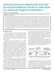
yacht. The graph <strong>of</strong> Fig. 4 shows the normalised total<br />
resistance components. For each speed the total<br />
resistance was normalised by dividing by the<br />
maximum total model scale resistance <strong>of</strong> the four runs<br />
for that speed.<br />
The model numbers refer to those given in<br />
Fig. 5, error bars have been drawn on this graph based<br />
on the random errors from repeatability tests. It can<br />
be seen from Fig. 6 that a large increase in resistance<br />
is obtained when the keel is added to the model for<br />
both cases <strong>of</strong> <strong>with</strong> and <strong>with</strong>out a rudder. Fig. 7 is a<br />
similar plot <strong>of</strong> normalised resistance for Rwp, the<br />
wave-pattern resistance.<br />
0.5<br />
0.25 0.3 0.35 0.4 0.45 0.5<br />
Fig. 8 Effect on Rt <strong>of</strong> adding appendages (Rt has been normalised)<br />
Fn<br />
Keel and Rudder, Model 1<br />
Keel Only, Model 3<br />
Rudder Only, Model 6<br />
No Keel, No Rudder, Model 5
1<br />
0.9<br />
0.8<br />
0.7<br />
0.6<br />
0.5<br />
0.25 0.3 0.35 0.4 0.45 0.5<br />
Fig. 9 Effect on Rwp <strong>of</strong> adding appendages (Rwp has been normalised)<br />
Fn<br />
Keel and Rudder, Model 1<br />
Keel Only, Model 3<br />
Rudder Only, Model 6<br />
No Keel, No Rudder, Model 5
From Fig. 10 it would appear that adding the<br />
rudder will nearly always result in a decrease in wavepattern<br />
resistance.<br />
Then taking the total resistance minus the wavepattern<br />
resistance we get the viscous resistance. A<br />
plot <strong>of</strong> the normalised viscous resistance has been<br />
shown in Fig. 11. The effect <strong>of</strong> adding a rudder can<br />
be seen to increase the viscous resistance, mirroring<br />
the results for the total resistance.<br />
The reduction <strong>of</strong> wave-pattern resistance by<br />
adding the rudder is thought to be due to the wave<br />
field created by the rudder, which appears to oppose<br />
the wave-pattern <strong>of</strong> the hull. This was tested<br />
theoretically by calculating the positions <strong>of</strong> the troughs<br />
and crests <strong>of</strong> a Kelvin wave-pattern produced by<br />
bodies positioned at the leading edges <strong>of</strong> the keel and<br />
rudder. A detailed description <strong>of</strong> the graphical<br />
method used to calculate crest lines for a Kelvin wavepattern<br />
can be found in Marr, 1994, pp 3-5. The<br />
position <strong>of</strong> the apex <strong>of</strong> the sectors containing the<br />
Kelvin wave-pattern was calculated from a guideline<br />
found in Newman, 1977 p 275, in which it is quoted<br />
that the apex should be upstream <strong>of</strong> the bow <strong>of</strong> a ship<br />
typically by one ship length. For the cases <strong>of</strong> the<br />
rudder and the keel one ship length was taken to be<br />
the length <strong>of</strong> the chord at the root <strong>of</strong> the foil. This<br />
1<br />
0.9<br />
0.8<br />
0.7<br />
0.6<br />
pattern was then superimposed on the wave-pattern<br />
determined from experiments. It was assumed that if<br />
either appendage created a trough where the main hull<br />
had a crest it would reduce the overall wave-pattern<br />
resistance. The conclusion from this analysis was that<br />
adding the keel should increase the wave-pattern<br />
resistance, because the crest lines from the keel<br />
generally lie on crest lines from the bare hull; whereas<br />
adding the rudder should reduce the wave-pattern<br />
resistance, because the crest lines lie on troughs from<br />
the bare hull. As stated above this is also the<br />
conclusion drawn from the wave-cut experiments.<br />
The rudder has more effect on the model <strong>with</strong> keel<br />
only (as compared <strong>with</strong> the bare model) because the<br />
waves are larger for this model and so interferences<br />
<strong>with</strong>in the wave-pattern have more effect.<br />
However, the addition <strong>of</strong> the rudder will also add<br />
to the viscous drag (both form drag and skin friction).<br />
In the runs shown above, except for the highest speed,<br />
the increase in Rv due to adding the rudder outweighs<br />
the decrease in Rwp. However, at full scale the<br />
relative importance <strong>of</strong> Rv is reduced slightly and so<br />
the trends in Rt could be reversed if the scale<br />
difference is large enough. For example the<br />
normalised total resistance plot <strong>of</strong> Fig. 12 plotted for<br />
full scale is reproduced in Fig. 13.<br />
0.5<br />
0.25 0.3 0.35 0.4 0.45 0.5<br />
Fig. 14 Effect on Rv <strong>of</strong> adding appendages (Rv has been normalised)<br />
Fn<br />
Keel and Rudder, Model 1<br />
Keel Only, Model 3<br />
Rudder Only, Model 6<br />
No Keel, No Rudder, Model 5
1<br />
0.9<br />
0.8<br />
0.7<br />
0.6<br />
0.5<br />
0.25 0.3 0.35 0.4 0.45 0.5<br />
Fig. 15 Full Scale Rt normalised<br />
1<br />
0.95<br />
0.9<br />
0.85<br />
0.8<br />
0.75<br />
0.7<br />
0.65<br />
0.6<br />
0.55<br />
Fn<br />
No Rudder, No Keel, Model 5<br />
Rudder Only, Model 6<br />
Keel Only, Model 3<br />
Keel and Rudder, Model 1<br />
0.5<br />
0.25 0.27 0.29 0.31 0.33 0.35 0.37<br />
Fig. 16 Rwp normalised for 20° heel 1° yaw<br />
Fn<br />
No Rudder, No Keel, Model 5<br />
Rudder Only, Model 6<br />
Keel Only, Model 3<br />
Keel and Rudder, Model 1
Heeled and yawed runs<br />
The conditions which were examined in detail<br />
were for heels <strong>of</strong> 10° and 20°, and yaws <strong>of</strong> 1°, 3° and<br />
5°. The same method for normalising the resistance<br />
was used, that is dividing by the largest resistance<br />
value for each Froude number on the graph. An<br />
example <strong>of</strong> the normalised wave-pattern resistance has<br />
been shown in Fig. 17 for 20° heel and 1° yaw. It<br />
would appear from the 12 runs presented in Fig. 18,<br />
and a further 60 similar runs (not shown here), that<br />
the wave-pattern resistance is reduced by adding the<br />
keel and increased by adding the rudder under some<br />
conditions. Clearly the simple rule <strong>of</strong> opposing wave<br />
fields is not working in these runs. The change in the<br />
flow velocity in the midships section due to the lift<br />
being produced by the keel has changed the trends in<br />
the wave-pattern resistance. However, creating<br />
similar flow changes around the stern would appear to<br />
produce different trends. Theoretical and<br />
experimental investigations have been carried out in<br />
other research upon wave-patterns <strong>with</strong>in which lift is<br />
being produced. For example wave-pattern research<br />
reported by Kuhn and Scragg, 1993, which was<br />
conducted on a surface piercing foil. This research<br />
found that the wave-pattern resistance would increase<br />
<strong>with</strong> increasing lift on a surface piercing foil. The<br />
increase in wave-pattern resistance between the foil at<br />
0° yaw and at 4° yaw was found to be about 60%,<br />
which was measured by wave-cut techniques and<br />
predicted <strong>with</strong> inviscid approximations. Therefore the<br />
reduction in wave-pattern resistance shown in Fig. 19<br />
<strong>with</strong> the addition <strong>of</strong> the keel is thought to be due to<br />
interference <strong>of</strong> the keel wave-pattern and that <strong>of</strong> the<br />
hull.<br />
Also, when the rudder is added to the bare hull<br />
the wave-pattern resistance only appears to change at<br />
the lowest speed (Fn = 0.286, full scale speed =<br />
5.50 knots), <strong>with</strong>in experimental error. For this speed<br />
the bare hull had an average <strong>of</strong> 13% less wave-pattern<br />
resistance for 10° heel 1° yaw, 20° heel 1° yaw and<br />
20° heel 3° yaw. The waves created by the keel in the<br />
above conditions would appear to be out <strong>of</strong> phase <strong>with</strong><br />
the yacht’s wave-pattern thereby reducing the overall<br />
resistance. However, if the rudder is added to the hull<br />
<strong>with</strong> the keel attached, the wave-pattern resistance is<br />
definitely increased. This would lead to the<br />
conclusion that adding the rudder only increases the<br />
wave-pattern resistance <strong>of</strong> the yacht when it is<br />
apparently out <strong>of</strong> phase <strong>with</strong> the waves created by the<br />
keel producing lift, thus adding to the waves created<br />
by the hull. The fact that the rudder decreases the<br />
wave-pattern resistance for the lowest speed and the<br />
small yaw angles for the bare hull would tend to<br />
indicate that the same phenomenon is apparent for<br />
these runs as is for the upright runs mentioned above.<br />
This is quite possible under the hypothesis presented<br />
in this paragraph as there is very little lift being<br />
produced for this condition.<br />
Fig. 20 is a graph <strong>of</strong> normalised total resistance<br />
for the same heeled and yawed condition.<br />
.
1<br />
0.95<br />
0.9<br />
0.85<br />
0.8<br />
0.75<br />
0.7<br />
0.65<br />
0.6<br />
0.55<br />
0.5<br />
0.25 0.27 0.29 0.31 0.33 0.35 0.37<br />
Fig. 21 Rt normalised for 20° heel 1° yaw<br />
Fn<br />
No Keel, No Rudder, Model 5<br />
Rudder Only, Model 6<br />
Keel Only, Model 3<br />
Keel and Rudder, Model 1
Here the total resistance would appear to be<br />
following much more predictable trends, in that<br />
adding an appendage increases the resistance, and<br />
adding the keel increases the resistance more than<br />
adding the rudder does. It is also worth noting that<br />
the changes in total resistance are much larger than<br />
1<br />
0.95<br />
0.9<br />
0.85<br />
0.8<br />
0.75<br />
0.7<br />
0.65<br />
0.6<br />
0.55<br />
those for the wave-pattern resistance. This would tend<br />
to suggest that the effect <strong>of</strong> adding appendages is<br />
mainly seen in the viscous resistance and the induced<br />
drag. The viscous resistance has been graphed in<br />
Fig. 22.<br />
No Keel, No Rudder, Model 5<br />
Rudder Only, Model 6<br />
Keel Only, Model 3<br />
Keel and Rudder, Model 1<br />
0.5<br />
0.25 0.27 0.29 0.31 0.33 0.35 0.37<br />
Fig. 23 Rv normalised for 20° heel 1° yaw<br />
1<br />
0.9<br />
0.8<br />
0.7<br />
0.6<br />
0.5<br />
0.4<br />
0.3<br />
0.2<br />
0.1<br />
Fn<br />
No Keel, No Rudder, Model 5<br />
Rudder Only, Model 6<br />
Keel Only, Model 3<br />
Keel and Rudder, Model 1<br />
0<br />
0.25 0.27 0.29 0.31 0.33 0.35 0.37<br />
Fig. 24 Calculated Di normalised for 20° heel 1° yaw<br />
Fn
Rv <strong>of</strong> Fig. 25 can be seen to be mirroring that <strong>of</strong> the<br />
total resistance.<br />
Fig. 26 shows the normalised induced drag,<br />
calculated using Equation ( 10 ). The vertical axis on<br />
this graph has been shifted relative to the previous<br />
graphs to give a zero origin. The graph appears very<br />
strange at first, because the highest induced drag is<br />
shown for the model <strong>with</strong> the keel only. An<br />
explanation for this must start <strong>with</strong> considering that<br />
the coefficient <strong>of</strong> induced drag Cdi is calculated using<br />
Equation ( 11 ). Therefore, an increase in induced<br />
drag is due to either an effective aspect ratio decrease<br />
or a lift increase. The calculated effective aspect ratios<br />
for the two models show a 30% change, however, the<br />
change in induced drag was <strong>of</strong> the order <strong>of</strong> 80%.<br />
Therefore the lift must have increased for Model 3.<br />
This was shown in the experimental results for the lift.<br />
For the lowest speed graphed in Fig. 24 the measured<br />
model scale lift for Model 3 was 6.78 N, whereas for<br />
Model 1 it was 3.36 N.<br />
Model 3 creating more lift than Model 1 appears<br />
to show an error, because Model 3 has less lifting<br />
surfaces than Model 1. However, the rudder is<br />
operating in the downwash <strong>of</strong> the keel and could<br />
therefore produce negative lift. This is also shown by<br />
the longitudinal centre <strong>of</strong> effort <strong>of</strong> the model, which is<br />
further forward for Model 1 than for Model 3. It was<br />
calculated (by inviscid theory, see Houghton and<br />
Brock, 1970, pp 370-374) that the downwash angle for<br />
this model is approximately equal to 70% <strong>of</strong> the angle<br />
<strong>of</strong> yaw, therefore at one degree yaw and one degree<br />
rudder angle relative to the yacht, the rudder is<br />
actually at 1.3° to the flow. To make negative lift the<br />
rudder is required to be at a negative angle to the flow,<br />
therefore either there is an error in the rudder setting<br />
or the assumptions required to calculate the downwash<br />
angle are not quite valid. The assumptions required<br />
are that the keel lift distribution is elliptic, that the<br />
rudder is located in the same plane as the wake <strong>of</strong> the<br />
keel (see Houghton and Brock, 1970, pp 371-372) and<br />
finally that the flow is not disturbed by the hull <strong>of</strong> the<br />
yacht.<br />
The final assumption has definitely been broken as the<br />
bare hull would appear to be capable <strong>of</strong> turning the<br />
flow towards the stern. This can be seen when<br />
examining the results for the hull <strong>with</strong> no keel and no<br />
rudder attached. For all <strong>of</strong> the heeled and yawed runs<br />
for this condition, using the sign convention shown in<br />
Fig. 27. A positive lift (along the y-axis) was<br />
measured <strong>with</strong> a negative yawing moment about the<br />
vertical axis. For most runs <strong>with</strong> the bare hull it is not<br />
possible to calculate <strong>with</strong> any accuracy the<br />
longitudinal centre <strong>of</strong> effort <strong>of</strong> the lift force. This is<br />
because <strong>with</strong> the errors on the lift measurement it is<br />
essentially zero, but the yaw moment is definitely<br />
negative. Therefore, the hydrodynamic forces on the<br />
hull create a pure moment on the hull (<strong>with</strong> no lift).<br />
There was, however, one extreme condition run for<br />
which it can be calculated that the longitudinal centre<br />
<strong>of</strong> effort is 4.7±2 m forward <strong>of</strong> the bow. Then by<br />
using a method described as slender body theory in<br />
Nomoto and Tatano, 1979, pp 76-80, a theoretical<br />
prediction for the centre <strong>of</strong> effort can be calculated.<br />
This calculation results in a predicted centre <strong>of</strong> effort<br />
<strong>of</strong> 3.73 m forward <strong>of</strong> the bow. Therefore, it can be<br />
concluded that the situation seen in the experiments is<br />
also predicted to a certain degree in theory.<br />
This is possible if the flow is turned around the<br />
yacht, thus providing a negative lift force on the stern<br />
<strong>of</strong> the yacht. The hypothesis can be better understood<br />
by examining the following two-dimensional<br />
schematic diagram.<br />
Fig. 28 Possible two-dimensional streamlines to<br />
give positive lift and negative yaw moment<br />
Fig. 29 is a view looking up at the bottom <strong>of</strong> the<br />
hull, and shows a possible set <strong>of</strong> streamlines in one<br />
plane which could give a positive lift and a negative<br />
yaw moment. This combination will then give a<br />
longitudinal centre <strong>of</strong> effort well forward <strong>of</strong> the bow,<br />
resulting in the yacht wanting to steer to windward, or<br />
weather helm. It is therefore possible to give the<br />
rudder negative lift, as seen in the results mentioned<br />
above.<br />
This feature was further investigated by<br />
examining the tests done for 20° heel and 5° yaw. For
this case it was concluded that the rudder was not<br />
generating negative lift, as the lift increased and the<br />
centre <strong>of</strong> effort moved aft for Model 1 when compared<br />
<strong>with</strong> Model 3. It is believed that there are two reasons<br />
for the difference. Firstly, the rudder would be<br />
coming out <strong>of</strong> the plane <strong>of</strong> the wake <strong>of</strong> the keel, thus<br />
reducing the velocity <strong>of</strong> the fluid from the tip and root<br />
vorticies <strong>of</strong> the keel, therefore reducing the downwash<br />
angle. Secondly the yacht is turning the flow at the<br />
stern less at higher angles <strong>of</strong> yaw.<br />
However, the use <strong>of</strong> a single post dynamometer<br />
makes the investigation <strong>of</strong> rudder lift difficult. This is<br />
because the yaw angle and the rudder angle are not<br />
known <strong>with</strong> high accuracy . Also the post can twist<br />
slightly due to the yaw moment experienced by the<br />
model. It is believed at this stage that the single post<br />
dynamometer has not introduced errors which affect<br />
the conclusions above. For these reasons the<br />
phenomenon described as negative lift on the rudder is<br />
the subject <strong>of</strong> further investigation.<br />
1<br />
0.9<br />
0.8<br />
0.7<br />
0.6<br />
Keel Rudder Separation Effects<br />
Upright runs<br />
Tests were carried out on three different models<br />
<strong>with</strong> varying keel rudder separation. Model 1 had the<br />
rudder in the design position, Model 2 had the rudder<br />
moved aft, and Model 4 had the rudder moved<br />
forward. The same analysis used above was carried<br />
out, resulting in the graph shown as Fig. 30 for the<br />
normalised wave-pattern resistance. The lowest speed<br />
seems to show very little change in wave-pattern<br />
resistance. The middle speed in the above graph<br />
shows the largest change in Rwp for the conditions<br />
considered. At this speed the rudder forward appears<br />
to have the lowest value for Rwp, which is thought to<br />
be due to smoothing the section area curve.<br />
Smoothing the section area curve is known to reduce<br />
the wave-pattern resistance, for example see Keuning<br />
and Kapsenberg, 1995, p 138. The same plot for total<br />
resistance is shown in Fig. 31.<br />
0.5<br />
0.25 0.27 0.29 0.31 0.33 0.35 0.37<br />
Fig. 32 Effect on Rwp <strong>of</strong> keel rudder separation (Rwp has been normalised)<br />
Fn<br />
Rudder Aft, Model 2<br />
Rudder Forward, Model 4<br />
Rudder in Design Position, Model 1
1<br />
0.9<br />
0.8<br />
0.7<br />
0.6<br />
0.5<br />
0.25 0.27 0.29 0.31 0.33 0.35 0.37<br />
Fig. 33 Effect on Rt <strong>of</strong> keel rudder separation (Rt has been normalised)<br />
The values plotted in Fig. 34 are extremely close<br />
together, therefore it can be assumed that at model<br />
scale the total resistance is not affected very much by<br />
keel rudder separation. A definite trend is evident<br />
1<br />
0.9<br />
0.8<br />
0.7<br />
0.6<br />
Fn<br />
Rudder Aft, Model 2<br />
Rudder Forward, Model 4<br />
Rudder in Design Position, Model 1<br />
suggesting that the further the rudder is moved aft the<br />
lower the total resistance will be. Fig. 35 is a plot <strong>of</strong><br />
the viscous resistance normalised <strong>with</strong> respect to the<br />
maximum value <strong>of</strong> the three models as above<br />
0.5<br />
0.25 0.27 0.29 0.31 0.33 0.35 0.37<br />
Fig. 36 Effect on Rv <strong>of</strong> keel rudder separation (Rv has been normalised)<br />
Fn<br />
Rudder Aft, Model 2<br />
Rudder Forward, Model 4<br />
Rudder in Design Position, Model 1
Again this graph mirrors that <strong>of</strong> the total<br />
resistance, as most <strong>of</strong> the resistance is viscous<br />
resistance for these runs. Typically the viscous<br />
resistance makes up between 80-90% <strong>of</strong> the total<br />
resistance for these runs. As mentioned previously the<br />
rudder tends to emerge at higher speeds, due to large<br />
trimming moments being applied, which could<br />
account for a lot <strong>of</strong> the reduction in viscous resistance.<br />
This goes against the general rule <strong>of</strong> thumb which<br />
says that the larger the buttock angle the larger will be<br />
the viscous resistance. By the above observations it<br />
would appear that the rudder emerging outweighs this<br />
usual effect.<br />
The largest changes are evident in the wavepattern<br />
resistance thus indicating that the wavepattern<br />
resistance is more sensitive to changing the<br />
keel rudder separation.<br />
Remaining Conditions<br />
The remaining conditions to be considered are<br />
all heeled and yawed runs for which the keel rudder<br />
separation was varied and the rudder angle was<br />
varied. To draw definite conclusions for these runs is<br />
very difficult as so many variables are changing which<br />
need to be considered. It is for these reasons that the<br />
analyses presented above shall not be presented for<br />
these series. To get a better appreciation <strong>of</strong> what is<br />
actually happening a more detailed picture <strong>of</strong> the flow<br />
around the yacht is required.<br />
Nevertheless the wave-pattern resistance shows a<br />
much greater difference than the total resistance when<br />
these conditions are changed. The viscous resistance<br />
constitutes the larger portion <strong>of</strong> the total resistance,<br />
and so it follows the trends <strong>of</strong> the total resistance. For<br />
example considering a low speed run, a change <strong>of</strong><br />
12% is evident in the wave-pattern resistance, whereas<br />
a change <strong>of</strong> only 2% is evident for the total resistance.<br />
In the analysis presented above the interaction<br />
effects on the lift <strong>of</strong> the yacht have not been discussed.<br />
However, the change in lift due to the variables<br />
examined has been included in the following VPP<br />
analysis.<br />
DESIGN GUIDELINES FROM CURRENT<br />
WORK<br />
The purpose <strong>of</strong> the research explained in this<br />
paper, as stated previously, is to provide design<br />
information as to the effects <strong>of</strong> hull-appendage<br />
interaction on resistance and performance. To<br />
accomplish this aim the final product must be an<br />
assessment <strong>of</strong> the relative performance effects <strong>of</strong> this<br />
interaction. The changes introduced as a result <strong>of</strong> this<br />
research have two main features. Firstly the resistance<br />
is scaled differently, and then the effects <strong>of</strong> the rudder<br />
variables are incorporated into the VPP.<br />
Scaling Modification Effects<br />
The changes in scaling when the wave-cut<br />
results are used have been explained above. It is<br />
sufficient here to realise that when using a traditional<br />
method <strong>of</strong> scaling, the wave-pattern resistance (here<br />
equated to the wave resistance) has been severely<br />
overestimated as compared <strong>with</strong> a wave-cut guided<br />
scaling method. Since the viscous resistance for a full<br />
scale prototype is less than the viscous resistance for a<br />
model, the total full scale resistance is reduced.<br />
Therefore the predicted velocity <strong>of</strong> the yacht will be<br />
increased. The average increase in yacht velocity was<br />
calculated to be 1.44%. From experience it is known<br />
that using tank results to predict full scale speed<br />
generally under-predicts the performance <strong>of</strong> the full<br />
scale yacht, the change to scaling methods presented<br />
here could therefore go to explain some <strong>of</strong> the<br />
difference.<br />
To get an overall picture <strong>of</strong> the yacht’s<br />
performance the General Purpose Rating (GPR) can be<br />
considered. This is a measure <strong>of</strong> a yacht’s<br />
performance calculated from the VPP results. The<br />
units <strong>of</strong> the GPR are seconds per nautical mile. The<br />
wind conditions are an average <strong>of</strong> results for 8 knots<br />
and 12 knots <strong>of</strong> true wind for a linear random (LR)<br />
course. The LR course is a standard course used in<br />
the IMS handicapping system, it consists <strong>of</strong><br />
considering that the yacht sails a straight course and<br />
that the wind angle varies for equal amounts <strong>of</strong> time<br />
between 0° and 180°. The calculated GPR figure<br />
shows a change <strong>of</strong> -2.5% when the wave-cut scaling<br />
procedure is used.<br />
Errors in performance indicators<br />
For the analysis presented here the most<br />
important errors are the random errors in the data.<br />
Systematic errors are <strong>of</strong> course important when<br />
considering the actual performance prediction,<br />
however these cannot be fully described <strong>with</strong>out more<br />
validation, such as full scale tests.<br />
A series <strong>of</strong> repeat runs was used to identify the<br />
random errors in the wave-pattern record. This gave<br />
an error <strong>of</strong> ±0.2 mm in the measured wave heights.<br />
Then the systematic errors were estimated for the<br />
wave-cut spacing measurement. These two errors<br />
were added to wave-pattern pr<strong>of</strong>iles as Gaussian<br />
random noise and the data was reanalysed, the<br />
difference between the results for the original data and<br />
the artificially corrupted data was taken to be the<br />
error. This procedure was repeated five times for each<br />
run investigated, <strong>with</strong> different random noise. It was
calculated that the known errors present in the wavepattern<br />
resistance due to incorrect readings were 1.5%.<br />
The regression process used to incorporate the results<br />
into the VPP, by virtue <strong>of</strong> the averaging nature <strong>of</strong><br />
regression, should help to reduce some <strong>of</strong> this error.<br />
Therefore it can be said that the total random error in<br />
resistance predictions should be less than 1.5%.<br />
If it is assumed that a percentage change in the<br />
resistance is linearly proportional to the resulting<br />
percentage change in performance indicator, then the<br />
maximum percentage errors in each performance<br />
indicator can be calculated. Using the cases presented<br />
above, an average change in total resistance <strong>of</strong> -11.6%<br />
resulted in an average velocity change <strong>of</strong> 1.4% and a<br />
GPR change <strong>of</strong> -2.5%. Therefore if an error <strong>of</strong> 1.5%<br />
was present in the total resistance value, this would<br />
correspond to an error <strong>of</strong> 0.2% in the velocity<br />
prediction and 0.3% in GPR.<br />
Rudder Variables Effects on <strong>Yacht</strong> Performance<br />
The effects on the yacht’s performance due to the<br />
rudder variables investigated were found to be very<br />
small. Typically the changes in velocity were <strong>of</strong> the<br />
order <strong>of</strong> less than 1%. Therefore it was considered the<br />
changes in velocity were too small to draw any<br />
meaningful conclusions from polar plots <strong>of</strong> the yacht<br />
velocity. Instead the calculated GPR (defined above)<br />
can be compared for each rudder variation.<br />
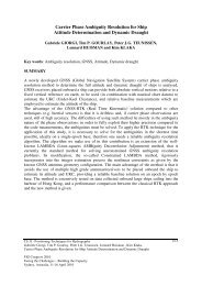
Worse<br />
performance<br />
%Change GPR from reference<br />
Better<br />
performance<br />
0.30%<br />
0.10%<br />
-0.10%<br />
-0.30%<br />
-0.50%<br />
-0.70%<br />
5<br />
4<br />
3<br />
Rudder Angle (degrees)<br />
2<br />
1<br />
It is important to run a base case for the yacht<br />
performance first, which gives the change in predicted<br />
performance due to the wave-cut scaling technique.<br />
This was done for the full scale yacht <strong>with</strong> a keel<br />
rudder separation <strong>of</strong> 4.75 m (measured from the<br />
leading edge <strong>of</strong> the keel to the leading edge <strong>of</strong> the<br />
rudder, positive in the aft direction) and a rudder<br />
angle equal to the yaw angle at all times. This<br />
condition corresponds to the design test condition.<br />
The way in which GPR changes <strong>with</strong> the two<br />
variables investigated is plotted in Fig. 37. In Fig. 38<br />
the rudder angle is relative to the centre line <strong>of</strong> the<br />
yacht. From this figure it can be concluded that<br />
moving the rudder aft from the design position will<br />
marginally improve the performance <strong>of</strong> the yacht, by<br />
just greater than the random error. Moving the rudder<br />
forward by the same amount has exactly the opposite<br />
effect. Keeping the rudder at an angle <strong>of</strong> 0° appears to<br />
improve the yacht’s performance by a marginal<br />
amount, whilst setting it to 5° appears to do the<br />
opposite. The greatest improvement is obtained by<br />
moving the rudder aft and reducing the rudder angle<br />
to 0°, whereas the worst performance is obtained by<br />
moving the rudder forward and setting the angle to 5°.<br />
0<br />
5.75<br />
5.35<br />
4.95<br />
4.55<br />
4.15<br />
3.75<br />
Full Scale Keel Rudder<br />
Separation (m)<br />
Fig. 39 Surface plot <strong>of</strong> % variation in GPR <strong>with</strong> rudder angle and keel rudder separation<br />
0.10%-0.30%<br />
-0.10%-0.10%<br />
-0.30%--0.10%<br />
-0.50%--0.30%<br />
-0.70%--0.50%
CONCLUSIONS<br />
Firstly for the test conditions which involved<br />
simply adding the appendages the total resistance<br />
follows fairly expected trends. For example adding<br />
the keel tends to increase the total resistance more<br />
than adding the rudder does. However, these trends<br />
are not evident in the wave-pattern resistance, because<br />
<strong>of</strong> the interference effects on the flow around the<br />
yacht. The expected trends are therefore due mainly<br />
to viscous and induced drag differences resulting<br />
simply from the increase in wetted area and associated<br />
form drag. The hull-appendage interference drag can<br />
therefore be better understood by wave-cut type<br />
analysis. Another approach has been taken in the past<br />
where an empirical formula is used to estimate the<br />
viscous interaction forces, see for example Teeters,<br />
1993.<br />
Trends <strong>with</strong>in the runs which involved changing<br />
appendage parameters were much more difficult to<br />
find. However, the changes were much more evident<br />
in Rwp than Rt or Rv, therefore appendage variations<br />
do actually show themselves more in the wave-pattern<br />
than in the total resistance which is dominated by<br />
viscous effects. The exact nature <strong>of</strong> the interference<br />
effects is difficult to decipher <strong>with</strong>out a greater<br />
knowledge <strong>of</strong> the flow patterns around the yacht.<br />
The stated aim <strong>of</strong> this project was to provide<br />
design information as to the effects <strong>of</strong> hull-appendage<br />
interaction on the performance <strong>of</strong> a sailing yacht. The<br />
assumption that the interaction forces would be most<br />
evident in the wave-pattern resistance was examined<br />
by conducting wave-cut experiments that are<br />
constructed to measure the resistance associated <strong>with</strong><br />
creating the inviscid wave-pattern produced by a<br />
model yacht. By showing that variables which should<br />
affect the interaction forces the most also result in a<br />
large change in wave-pattern resistance relative to the<br />
total resistance, it has been reasoned that this<br />
assumption was correct.<br />
Regardless <strong>of</strong> the reasoning, the question still<br />
remains as to whether or not design information has<br />
been provided. The answer to this question lies in the<br />
work presented concerning the performance<br />
indicators, in which it is concluded that varying the<br />
rudder angle and the keel rudder separation suggests<br />
that the rudder should be put as far aft as possible and<br />
the rudder angle should be set as low as possible.<br />
ACKNOWLEDGMENTS<br />
This paper is based on research conducted as a<br />
part <strong>of</strong> the Australian Maritime Engineering CRC’s<br />
<strong>Yacht</strong> Technology and Performance research program.<br />
The authors would like to thank the following<br />
for their help during experiments and data analysis<br />
Giles Thomas, Bruce McRae, Roy Horne, Martin<br />
Shaw, Mark Lees, Damien Freeman, Ben Church and<br />
Warwick Oliver.<br />
REFERENCES<br />
Binns, J. “<strong>Hull</strong>-<strong>Appendage</strong> <strong>Interaction</strong> <strong>of</strong> a Heeled and<br />
Yawed Vessel”, to be submitted for MSc Thesis,<br />
Curtin University <strong>of</strong> Technology, 1996<br />
Duncan, W.J., Thom, A.S., and Young, A.D.,<br />
Mechanics <strong>of</strong> Fluids, Edward Arnold, London, 1970<br />
Eggers, K.W., Sharma, S.D., Ward, L.W., “An<br />
Assessment <strong>of</strong> Some Experimental Methods for<br />
Determining the Wavemaking Characteristics <strong>of</strong> a<br />
Ship Form”, Trans SNAME, 75, 1967, pp 112-157<br />
Gerritsma, J., Keuning, J.A. and Versluis, A., “<strong>Sailing</strong><br />
<strong>Yacht</strong> Performance in Calm Water and Waves”, The<br />
11th Chesapeake <strong>Sailing</strong> <strong>Yacht</strong> Symposium, 1993,<br />
pp 233-245<br />
Harvald, S.A., Resistance and Propulsion <strong>of</strong> Ships,<br />
Wiley-Interscience, New York, 1983<br />
Hogben, N. and Standing, R.G., “Wave Resistance<br />
from Routine Model Tests”, Trans. RINA, 1974,<br />
pp 279-295<br />
Houghton, E.L. and Brock, A.E., Aerodynamics for<br />
Engineering Students, Edward Arnold, London, 1970<br />
Hughes, G., “An Analysis <strong>of</strong> Ship Model Resistance<br />
into Viscous and Wave Components Parts I and II”,<br />
Trans. RINA, 108, 1966, pp 289-302<br />
Keuning, J.A. and Kapsenberg, G.K., “Wing-Body<br />
<strong>Interaction</strong>s on a <strong>Sailing</strong> <strong>Yacht</strong>”, The 12th<br />
Chesapeake <strong>Sailing</strong> <strong>Yacht</strong> Symposium, 1995, pp 133-<br />
144<br />
Kuhn, J.C. and Scragg, C.A, “Analysis <strong>of</strong> Lift and<br />
Drag on a Surface-Piercing Foil”, The 11th<br />
Chesapeake <strong>Sailing</strong> <strong>Yacht</strong> Symposium, 1993, pp 277-<br />
288<br />
Marr, G., “An Introduction to the Computation <strong>of</strong><br />
Wave Resistance for <strong>Yacht</strong> Design”, The International<br />
<strong>Yacht</strong> Design Symposium, 1994<br />
Newman, J.N., Marine Hydrodynamics, MIT Press,<br />
London, 1977
Nomoto, K. and Tatano, H., “Balance <strong>of</strong> Helm <strong>of</strong><br />
<strong>Sailing</strong> <strong>Yacht</strong>s”, HISWA <strong>Sailing</strong> <strong>Yacht</strong> Symposium,<br />
1979, pp 65-89<br />
Rosen, B.S., Laiosa, J.P., Davis, W.H. and<br />
Stavetski, D., “SPLASH Free-Surface Flow Code<br />
Methodology for Hydrodynamic Design and Analysis<br />
<strong>of</strong> IACC <strong>Yacht</strong>s”, The 11th Chesapeake <strong>Sailing</strong> <strong>Yacht</strong><br />
Symposium, 1993, pp 35-49<br />
Teeters, J.R., “Refinements in the Techniques <strong>of</strong> Tank<br />
Testing”, 11th Chesapeake <strong>Sailing</strong> <strong>Yacht</strong> Symposium,<br />
1993, pp 13-34<br />
APPENDIX A: SUMMARY OF WAVE-CUT<br />
PROCEDURES<br />
The methods by which the figures presented in<br />
this paper have been calculated are detailed in Binns,<br />
1996. The following is a brief description <strong>of</strong> how the<br />
wave-cut results can be obtained, <strong>with</strong>out any pro<strong>of</strong>s<br />
or error estimates.<br />
Probe Spacing<br />
Longitudinal cuts were performed using 8<br />
channels <strong>of</strong> capacitance wave probes across the testtank.<br />
The position <strong>of</strong> the probes from the start <strong>of</strong> the<br />
run was 45 m and the spacing between the probes was<br />
set as close to the tank width divided by ten as<br />
possible. The cut spacing was suggested by Hogben<br />
and Standing, 1974, p 295, however it was felt that it<br />
would be better to try and place at least one cut at the<br />
position <strong>of</strong> the tank width on four. This conclusion<br />
was reached by examining which wave-number<br />
component <strong>of</strong> the total resistance was always very<br />
large, and then calculating which position should<br />
measure the greatest change in this wave-number<br />
component. To check this hypothesis more tests<br />
would have to be conducted, <strong>with</strong> a probe positioned at<br />
this spacing.<br />
It is worth noting here that the probe spacing<br />
should be measured as accurately as possible. Serious<br />
systematic errors can be introduced if this is not done.<br />
An acceptable accuracy for this measurement would be<br />
±1 mm.<br />
Data acquisition<br />
It is considered that the signals were adequately<br />
filtered, through use <strong>of</strong> carefully designed analog and<br />
digital filters. The number <strong>of</strong> samples to be taken for<br />
each run can be calculated from the following<br />
equation<br />
N A LWL<br />
= × R + B,<br />
( 12 )<br />
Vs<br />
where LWL is the waterline length <strong>of</strong> the model in<br />
metres, Vs is the model speed in m/s, R is the sample<br />
rate in Hz and A and B are coefficients. The<br />
coefficient A is the number <strong>of</strong> boat lengths to use (here<br />
taken as 6), and B is the number <strong>of</strong> samples which are<br />
redundant (here taken as 600).<br />
Multiple Longitudinal Cut Method Used<br />
The method used to calculate the wave-pattern<br />
resistance is best described as a least squares multiple<br />
longitudinal cut method. A summary <strong>of</strong> the procedure<br />
follows.<br />
Symmetric Analysis<br />
Through consideration <strong>of</strong> the wave potential <strong>of</strong> a<br />
Kelvin wave-pattern it can be shown that the wave<br />
heights can be described by the following equation<br />
1<br />
ζ(<br />
x, y)<br />
=<br />
2<br />
where,<br />
n=∞<br />
∑<br />
n=−∞<br />
( α )<br />
( α )<br />
⎛ A n cos nx<br />
⎞<br />
⎜<br />
⎟ cos<br />
⎝+<br />
B sin x<br />
⎟<br />
⎠<br />
n n<br />
( β y)<br />
n<br />
,<br />
( 13 )<br />
α n = γ n cos θ n ,<br />
nπ<br />
β n =<br />
b<br />
2<br />
, ( 14 )<br />
γ<br />
2<br />
cos θ = K tanh γ h,<br />
n n n<br />
g<br />
K = ,<br />
2<br />
Vs<br />
and<br />
π<br />
Ksinθ n sec θ<br />
2 2n<br />
n = .<br />
b<br />
In the above expressions θn is the propagation<br />
angle <strong>of</strong> the nth wave component, b is the tank width,<br />
Vs is the vessel velocity and g is the acceleration due<br />
to gravity. Then a least squares solution to<br />
Equation ( 15 ) can be calculated from model wave<br />
heights obtained. The total wave-pattern resistance<br />
can be calculated from<br />
⎡<br />
2 ⎛ Q K ⎞<br />
⎤<br />
0 2 2<br />
⎢2⎜2<br />
− ⎟ ( A + B ) ⎥<br />
2 0 0<br />
ρgb<br />
⎢ ⎝ α 0 ⎠<br />
⎥<br />
Rwp = ⎢<br />
⎥ ,<br />
8 ∞<br />
2<br />
⎢ ⎛ Q nK<br />
⎞ 2 2<br />
+ ⎜ − ⎟ ( A n + B<br />
⎥<br />
⎢ ∑ 2<br />
2<br />
n )<br />
⎣ n ⎝ n ⎠<br />
⎥<br />
= 1 α<br />
⎦<br />
( 16 )<br />
where,
Q n = tanh 2 ⎡ 2γ nh ⎤<br />
γ nh 1+<br />
⎣ ⎢ sinh 2γ nh ⎦ ⎥ .<br />
Asymmetric Analysis<br />
It can be shown that an asymmetric wave-pattern<br />
can be described by the following equation<br />
n=∞<br />
1 ⎛A<br />
n cos(<br />
α nx)<br />
⎞ ⎛ b<br />
ζ(<br />
x, y)<br />
= ⎜<br />
⎟<br />
⎛ ⎞⎞<br />
cos β n y<br />
⎝+<br />
B sin α x<br />
⎟ ⎜ ⎜ − ⎟⎟<br />
2 ∑<br />
⎠ ⎝ ⎝ 2⎠<br />
⎠<br />
n=−∞<br />
( )<br />
n n<br />
( 17 )<br />
then the same equations can be used as for the<br />
symmetric analysis <strong>with</strong> the exception <strong>of</strong><br />
Equation ( 18 ), which becomes<br />
β<br />
nπ<br />
= . ( 19 )<br />
n<br />
It can be seen that odd values <strong>of</strong> n in<br />
Equation ( 20 ) describe asymmetric waves and even<br />
values describe symmetric waves. The asymmetric<br />
analysis can therefore also be used for symmetric<br />
patterns, however this is inadvisable as extremely illconditioned<br />
matrices result from the least squares<br />
analysis.<br />
b