investigation of underwater acoustic multi-path doppler and delay ...

INVESTIGATION OF UNDERWATER ACOUSTIC 

MULTI-PATH DOPPLER AND DELAY SPREADING 

IN A SHALLOW MARINE ENVIRONMENT 

Michael Caley and Alec Duncan 

Curtin University, Department of Imaging and Applied Physics, Centre for Marine Science and Technology, Perth, Australia 

michaelcaley@westnet.com.au 

Doppler frequency spreading and arrival delay spreading of underwater acoustic communication signals under the influence 

of surface waves and transmitter-receiver motion were investigated in a channel probing experiment conducted primarily 

with binary pseudo-noise (PN) sequences ranging from 21ms to 1.4s duration. Testing was conducted in a 13.5m deep 

environment at transmission distances ranging from 44m to 1007m. The channel Doppler response was investigated both 

by time-domain Doppler search of the transmit-receive correlation for successive repeats of a 1.4s probe sequence, and by 

Fourier analysis of the channel impulse response history from a repeated 21ms probe sequence (i.e. Spreading Function). 

The bounds of Doppler shift imparted by relative transmitter/receiver motion and surface wave motion to idealised soundray 

transmission paths has been compared with experimental Doppler indicated by the Spreading Function. The coherence 

of the experimental channel response was also examined for different propagation ranges and at different delayed arrivals 

of the experimental signals. 

INTRODUCTION 

The choice for the wireless transmission of data underwater 

is between electromagnetic waves (e.g. light or radio) or sound 

waves. Light and radio waves are valuable for high-rate data 

transmission through water over short ranges of the order 

of a few metres. When transmission is required over longer 

distances through water, sound waves are the only viable 

wireless option. 

Underwater acoustic data transmission is not without 

signifi cant constraints intrinsic to the marine environment. 

The underwater acoustic environment is highly reverberant, 

resulting in multiple refl ected copies of any transmitted signal 

arriving at the receiver at delayed intervals (delay spreading), 

and with the relative delays generally changing with time. The 

frequency of transmitted signals is also signifi cantly distorted 

by transient Doppler effects generated by elongation and 

contraction of surface refl ected transmission paths (Doppler 

frequency spreading), or Doppler frequency shifts from 

movement of either (or both) the transmitter and receiver. 

Transient delay spreading and Doppler spreading of the 

received signal present signifi cant challenges to the decoding 

of incoming data symbols by a communications receiver, 

with the problem becoming more diffi cult as the rate of data 

transmission increases. 

In 2011 the Department of Electrical and Computer 

Engineering and the Centre for Marine Science and Technology 

(CMST) at Curtin University commenced a project to develop 

high-rate underwater acoustic communications to support 

developing ocean-based industries in Australia [1]. The authors’ 

role is to develop an underwater acoustic communication 

channel simulator to support this project. The purpose of the 

simulator is to simulate the way that the real ocean produces 

transient distortion of acoustic communication signals between 

a transmitter and a receiver, including interference effects from 

highly variable natural and anthropogenic noise. The simulator 

provides a confi gurable analogue of the real ocean that can be 

used to improve understanding of the infl uence of the marine 

acoustic environment on communications signals, and assists 

the development of underwater communication modulation 

and demodulation algorithms and hardware. 

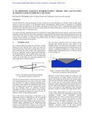
Transient phenomena that are key to the development of an 

acoustic channel simulator for high-rate data communications 

are the transient delay and Doppler frequency spreading of the 

received signal imparted by the moving sea-surface, shown 

schematically in Fig. 1, and the transient Doppler imparted by 

moving transmitter and/or receiver platforms [2,3]. 

Figure 1. Conceptual signal Doppler shift and path delay 

Experimental channel probing was conducted primarily 

with binary pseudo-noise (PN) sequences ranging from 21ms 

to 1.4s duration. The signal was created by phase-modulating 

a continuous 12kHz sinusoid with the binary sequence. This 

method is described in communication literature as Direct 

Sequence Spread Spectrum (DSSS) signalling. 

In this investigation the channel Doppler response to probe 

20 - Vol. 41, No. 1, April 2013 Acoustics Australia

signals was investigated both by a time-domain resampling 

Doppler search method on successive transmit-receive (txrx) 

PN sequence blocks, and also by Fourier analysis of the channel 

response with respect to time, to generate the frequencydomain 

Doppler Spreading Function. 

It is customary to present the channel Doppler axis of 

the Spreading Function S(τ,f) in the units of Hz. S(τ,f) was 

calculated in Eq. (1) by discrete Fourier analysis of the channel 

response h(τ,t). 

n=0 i2πnp 

S (τ,f) = ∑ h(m,n)exp (- ) 

(1) 

n=N-1 N 

S(τ,f) was calculated from N = 1400 impulse responses h(τ,t) 

spaced in the time (t) dimension at intervals T = 21ms, with 

time t = nT. The impulse response in the delay dimension (τ) 

was calculated from sampling at frequency fs = 96kHz, with 

response delay τ = m/fs and Doppler frequencies f = p/NT 

where p ϵ [-N/2+1,...,N/2]. 

When the complex channel response h(τ,t) is determined by 

cross-correlation of a modulated transmit and receive signal, 

the rate at which the phase of h(τ,t) changes with respect to 

time (t) is scaled by the probe signal carrier frequency (f0 ). 

Accordingly the Doppler shift spectrum at each delay (τ) 

calculated by DFT of h(τ,t) is also scaled by the probe signal 

carrier frequency. 

For a physical layer modeller it is helpful to note that the 

Doppler shift derived by (1) is responsive to h(τ,t) phase changes 

originating not only from Doppler phase compression/dilation, 

but also from what will be described as ‘apparent’ Doppler due 

to phase changes associated with transient phase interference 

of clustered multipath arrivals, and transient angular scattering 

of propagation paths by a moving sea surface [4]. 

The channel Doppler response may be expressed either 

as an equivalent velocity shift δv or as an equivalent signaldependent 

frequency shift δf as linked by Eq. (2), where positive 

δv represents an equivalent velocity shift that contracts the 

propagation path length and c is the speed of sound in water. 

δf(f 0 ) = δv/c (2) 

In this paper the measured channel Doppler response has 

generally been reported as a frequency shift (Hz), but in the 

case of Spreading Function plots a secondary axis with Doppler 

velocity shift was added to enable comparison with Doppler 

velocity shift estimates from geometrical considerations. 

CHANNEL PROBING TESTS 

A shallow (13.5m) channel probing experiment was 

conducted in April 2012 over distances ranging from 44m 

to 1007m. The transmitter and receiver arrangements are 

illustrated in Figs. 2 and 3, respectively. The transmitter was 

inverted (relative to conventional vertical downwards primary 

axis alignment) to maximise the signal strength for surface 

refl ected transmission paths. 

Figure 2. Transmitter configuration 

Figure 3. Receiver configuration 

Experimental arrangement and instrumentation 

Transmitted and received signals were sampled with 24 bit 

resolution at 96kHz. Directional surface wave data was 

obtained from a Directional Wave Rider Buoy (DWRB) 

located approximately 1.5km NE of the receiver. The soundspeed 

profi le at each site was sampled with a Conductivity 

Temperature Depth (CTD) probe. The vessel was fi tted with 

pitch, heave and roll data acquisition sampling at 100Hz. Five 

temperature loggers sampling at 60 second intervals were 

suspended from the surface fl oat line. Grab samples were 

collected of the sandy bottom material. 

Probe signals 

Probe signals for simultaneous Doppler shift and delay 

detection consisted of a 12kHz continuous wave (CW) 

carrier modulated at a 3kHz chipping rate by binary phase 

pseudorandom (PN) sequences. The longer temporal effects 

Acoustics Australia Vol. 41, No. 1, April 2013 21

associated with wave and swell were explored by continuing 

the sequence repetitions over an interval greater than the swell 

period. A repeated pattern was transmitted consisting of 60s of 

1.4s PN sequence (n-bits = 4095), 30s of 170ms PN sequence 

(n-bits = 511) and 30s of 21ms PN sequence (n-bits = 63). 

This was followed by 30 repeats of a 16ms 8kHz-16kHz linear 

frequency sweep at 1s intervals. The sweeps were utilised to 

provide an unambiguous check on the channel delay spread 

and structure. 

The bandwidths of trial signals were guided by the ±3dB 

transmit sensitivity of the Chelsea Technologies CTG052 

transmit transducer. Signals were written to a 24 bit wav fi le 

then replayed on a digital audio player with output amplifi cation 

to the transmitter. 

Doppler and delay resolution – single block processing 

The delay resolution δt of multi-path arrivals for a PN probe 

signal is determined by the sequence chipping interval tchip as 

per Eq. (3). For a linear frequency sweep, δt is the inverse of 

the maximum sweep frequency. 

tchip δt = 

2 

(3) 

The Doppler velocity shift resolution δv for a PN sequence 

probe signal depends on the sequence repeat interval T and the 

signal carrier frequency f0 as per Eq. (4) where c is the speed 

of sound. For a linear frequency sweep, f0 is replaced by the 

maximum sweep frequency. 

c 

δv = 

f0T (4) 

The probe signal frequencies, repeat intervals, bandwidths 

and associated delay and Doppler resolutions are detailed in 

Table 1. 

Signal 

type 

f 0 

(kHz) 

Table 1. Trial test signals 

Period 

T (s) 

Chipping 

rate 

δ t 

(ms) 

δ v 

(m/s) 

PN 12 1.4 3 0.16 0.094 

PN 12 0.17 3 0.16 0.75 

PN 12 0.021 3 0.16 6.1 

Sweep 8-16 0.016 - 0.06 6.0 

Doppler resolution – 21ms ensemble block processing 

The Doppler velocity resolution of the Spreading Function 

from the 21ms probe impulse response history is also calculated 

by Eq. (4), but with T evaluated with the block ensemble 

duration of 30s. The resultant Doppler resolution is 0.0043m/s, 

or 0.033Hz, with Nyquist frequency of 23.8Hz. 

Test sea conditions 

The water column was well mixed during testing with 

the sound speed ranging almost linearly from 1537m/s at the 

surface to 1536m/s at the bottom. Wind conditions were light 

to still, with low swell and sea conditions reported at 15 minute 

intervals from the nearby (1.5km distant) Cottesloe Directional 

Wave Rider Buoy (DWRB) as summarised in Table 2. The 

appearance of the sea surface during testing is illustrated in 

Fig. 4. It is notably free of surface bubbles. 

Wave type 

Table 2. Wave height data for presented results 

Significant 

height H s 

Wave period 

T m 

Wave 

frequency 

Swell 0.4m 13-14s 0.07Hz 

Sea 0.25m 3s 0.33Hz 

Figure 4. Experimental sea surface 

IDEALISED CHANNEL DELAY STRUCTURE 

The arrival delay structure for an idealised ocean waveguide 

with specular surface and bottom refl ections and constant 

sound speed shown schematically in Fig. 5 is graphed in Fig. 6 

to assist with the interpretation of the measured delay structure. 

‘B’ stands for a bottom-bounce, and ‘S’ a surface-bounce. It 

may be noted that at increasing ranges the time separation 

between delays becomes less than the delay resolution of test 

signals listed in Table 1. 

Figure 5. Low order reflected paths 


Figure 6. Idealised delay structure of reflected paths relative to the 

direct path 

DOPPLER CONTRIBUTIONS FROM 

RELATIVE MOTION 

The primary geometrical sources of relative motion that 

contribute to the experimental Doppler shift are sea-surface 

motion, wave orbital motion coupling to the suspended 

transmitter, and transmitter movement generated by vessel 

rolling and drift as illustrated in Fig. 5. These components were 

resolved into the idealised acoustic transmission paths, then 

combined to provide a Doppler velocity shift interpretation 

of the Doppler effect indicated by the experimental Spreading 

Function. 

The slow-changing contributions (drift and swell orbital 

motion) have been treated as constant values, whereas the 

rapidly changing stochastic Doppler velocity contributions 

from sea-surface refl ections and vertical transmitter oscillation 

have been quantifi ed as 3σ estimates where σ is the standard 

deviation. Successive surface refl ections and vertical 

transmitter oscillations have been treated as independent 

processes. Only the vertical motion of surface refl ections has 

been considered. The more complex horizontal surface-wave 

velocity components are not considered. 

Vessel drift closing speed 

The average closing speed Vdrift was calculated from GPS 

data for the vessel drift. This speed ranged from 0.11m/s to 

0.19m/s for the data presented. This relative motion contributes 

almost the same Doppler shift to all transmission paths as per 

Eq. (5), where θ is the path launch angle from horizontal. 

V d = V drift cosθ (5) 

Transmit-receive motion coupled to orbital wave motion 

The cable tether of both the transmitter (tx) at 10m depth 

and the receiver (rx) hydrophone 1m off the bottom make both 

susceptible to orbital wave motion, however the movement of 

the receiver hydrophone would be limited compared to that of 

the transmitter. At the depth of the transmitter the horizontal 

component of swell orbital motion is signifi cant in the shallow 

test channel, with the contribution from wind-waves not 

extending below mid-depth. If it is conservatively assumed that 

the transmitter is completely compliant horizontally, the relative 

horizontal orbital motion Vorbital is calculated at up to 0.17m/s 

for the Table 2 data. This relative motion contributes almost the 

same Doppler to all transmission paths as per Eq. (6). 

Vo = Vorbital cosθ (6) 

Surface vertical velocity 

The maximum vertical surface velocity Vsurface at the point 

of surface refl ections was estimated based on the 3σ wave 

height for swell and sea by Eq. (7), providing estimates of 

0.39m/s for the Hs = 0.25m sea-waves, and 0.13m/s for the 

Hs = 0.4m swell. The higher estimate obtained from the windwaves 

was utilised as an upper bound estimate of Vsurface . The 

vertical surface motion from a single surface refl ection can be 

resolved in the direction of an idealised surface-refl ected path 

as per Eq. (8). 

Vsurface = 3πHs /2Tm (7) 

V s = 2V surface sinθ (8) 

Vertical transmitter motion 

The vertical velocity spectral density of the transmitter in 

Fig. 7 was calculated from the combined vessel pitch, heave 

and roll data by averaging 18 x 160s blocks of data with 

Hamming windowing. This data shows a peak at 0.07Hz that 

corresponds to the DWRB swell data, and peaks at frequencies 

similar to the DWRB data for wind-driven surface waves. 

These higher frequency peaks were likely infl uenced by the 

resonant pitch and roll frequencies of the vessel. The vertical 

root-mean-square (RMS) velocity from the data in the 0-2Hz 

range was 0.13m/s, providing a 3σ estimate of 0.39m/s for this 

component. 

−50 

0 0.5 1 

Frequency (Hz) 

1.5 2 

Figure 7. Transmitter vertical velocity power spectrum 

Acoustics Australia Vol. 41, No. 1, April 2013 23 

Power spectral density(dB m 2 s −2 /Hz) 

0 

−10 

−20 

−30 

−40

The vertical transmitter velocity Vtvert can be resolved in 

the direction of all surface and/or bottom refl ected transmission 

paths as per Eq. (9). 

Vt = Vtvert sinθ (9) 

Combination of geometrical Doppler velocity components 

resolved in path 

An estimate of the 3σ total in-path Doppler shift for a path 

involving nb surface bounces was calculated from components 

assuming independence of stochastic processes as per Eq. (10). 

Vtotal = Vd + Vo + √ Vt 2 + nbV 2 

s (10) 

Figure 8. 3σ estimates of maximum geometrical Doppler velocity 

shifts resolved along idealised paths for path delays < 10ms 

The geometrical Doppler components discussed in previous 

sections are compared in Fig. 8 for all idealised ray paths 

within 10ms delay relative to the direct path, for the example 

test distances of 110m, 500m, 1007m. The experimental txrx 

drift rate varied at each distance. Records of wave conditions 

from the nearby DWRB were comparable for all transmission 

ranges. This analysis indicates that the potential maximum 

in-path Doppler shift increases signifi cantly with the number 

of surface bounces at short range, with the vertical surface 

Doppler delay per surface bounce diminishing with range. 

It is noted that the test results relate to relatively low 

experimental surface wave heights as per Table 2. Sea and swell 

are commonly 4-5 times higher at the test site which would 

lead to all related Doppler velocity components increasing 

commensurately. 

EXPERIMENTAL DELAY RESULTS 

The transmit-receive correlation versus delay histories 

are presented for 110m, 500m and 1007m transmit ranges in 

Figs. 9-11. The correlation response for each time block was 

normalised by the product of the transmit and receive signal 

power. The plots are the absolute value of the correlation R, so 

do not reveal the phase changes occurring in R with time. 

Successive block impulse responses were aligned on the 

fi rst correlation maxima (with a 0.01ms numerical time step), 

without resampling to adjust for cyclical Doppler shift from 

txrx movement. Consequently the resultant channel response 

history will include distortion of the delay between the fi rst 

maxima and subsequent arrivals due to this txrx relative 

movement. However the magnitude of this delay distortion 

is less than 0.01ms, less than a tenth of the delay resolution 

for the experimental probe signal. It is concluded that the 

‘approximate’ delay history obtained in this manner is reliable. 

The correlation results from 16ms frequency sweeps at 1s 

intervals (not shown) were used to check on the delay structure 

out to 60ms, confi rming that the 10ms delay structure revealed 

by the 21ms probe sequence contains the signifi cant arrivals 

for this channel. 

Utilising the idealised delay structure in Fig. 6 for 110m 

range for reference, the fi rst correlation maximum in Fig. 9 

represents the combined direct and bottom-refl ected paths, 

with the second group of arrivals extending between 1ms and 

3ms corresponding to Surface, BS, SB and BSB refl ected paths. 

The next group of arrivals for paths involving two surface 

refl ections are apparent between 6ms and 10ms. 

At 500m range (Fig. 10) the contracting of the delay spread 

is apparent with two additional bands of higher order surface 

refl ections evident. The results at this range are notable as the 

fi rst correlation maximum is suppressed relative to the second 

as a consequence of destructive phase interference between the 

Direct and Bottom paths. In this channel the Surface, SB, BS 

and BSB paths combine to provide a stronger arrival, but with 

interruption at intervals matching the swell period, presumably 

relating to destructive interference associated with differential 

path elongation/contraction. 

At 1007m range the relative phases of the Direct, Surface 

and Bottom bounce again combine constructively to produce a 

strongest fi rst correlation maximum. 


Figure 9. Normalised txrx correlation history (dB)–21ms PN sequence 

@ 110m 

Figure 10. Normalised txrx correlation history (dB)–21ms PN 

sequence @ 500m 

Figure 11. Normalised txrx correlation history (dB)–21ms PN 

sequence @ 1007m 

EXPERIMENTAL DOPPLER SHIFT 

RESULTS 

Spreading Function Doppler Shift Indication 

The Spreading Functions corresponding to the 110m, 500m 

and 1007m ranges are presented in Figs. 12-14. The Spreading 

Functions are over-plotted with white markers representing the 

3σ Doppler estimates from geometrical consideration as per Fig. 

8, making use of the correspondence between Doppler frequency 

shift and velocity shift in Eq. (2). The corresponding delays of 

the white markers relate to an idealised waveguide with parallel 

boundaries. In reality the delays will vary with the path elongation 

and contraction associated with vertical surface movement, and 

with the moving refl ection position linked to travelling surface 

waves. The variation in actual delay of surface-interacting paths is 

indicated by the substantial delay-spreading (x-axis) evident in the 

Spreading Function compared to the idealised discrete delay points. 

Figure 12. Spreading Function (dB) with 3σ geometrical Doppler 

estimates @ 110m 



Acoustics Australia Vol. 41, No. 1, April 2013 25

The 3σ estimates of total Doppler velocity shift from relative 

movement on idealised transmission paths and a simplistic treatment 

of surface wave movement readily account for Doppler shifted 

arrivals within 25dB-30dB of the strongest arrival at all delays. This 

Doppler estimate from velocity shift is therefore considered useful 

to interpretation of the Spreading Function Doppler. 

Time domain Doppler search method 

The results presented below relate to approximately the 

same channel as the 110m results in Fig. 9 and Fig. 12, but 

with transmitter drift extending the average range to 122m, and 

reducing the averaging closing speed from 0.19m/s to 0.13m/s. 

Comparison of the short PN-sequence channel response history 

in Fig. 9 with the long PN-sequence channel response history in 

Fig. 15 illustrates how time varying channel Doppler degrades the 

txrx correlation for a relatively long 1.4s Doppler-sensitive sequence. 



Figure 15. Normalised txrx correlation (dB)–1.4s PN sequence @ 122m 

The correlation versus Doppler and time results presented 

in Figs. 16, 17 and 18 have been generated by block-by-block 

Doppler search for delay ranges relating to the fi rst, second 

and third delayed path groups illustrated in Fig. 15. Whilst not 

shown, the equivalent Doppler frequency range of these fi gures 

is ± 10 Hz, as for the short-sequence spreading function plots. 

The ‘ripples’ either side of the correlation maximum in Fig. 

16 result from the ambiguity function Doppler side-lobes of the 

1.4s PN sequence. The cyclical infl uence of swell orbital motion 

on relative motion is apparent in the Doppler time history for the 

fi rst, second and third delay arrival groups. This time-dependent 

Doppler information is not obtainable from the Spreading 

Function or the time-domain channel response for the short 21ms 

sequence, for which the Doppler resolution of 6.1m/s is too coarse 

to enable detection of Doppler shift from orbital motion. 

It appears from the time-domain Doppler analysis that there 

are no strong signal arrivals at large Doppler shift, however this 

Figure 16. First arrivals normalised correlation (dB) versus time and 

Doppler, 1.4s PN sequence @ 122m 

Figure 17. Second arrivals normalised correlation (dB) versus time 

and Doppler, 1.4s PN sequence @ 122m 


Figure 18. Third arrivals normalised correlation (dB) versus time and 

Doppler, 1.4s PN sequence @ 122m 

does not exclude the possibility of such transients occurring at 

a signifi cantly shorter time-scale than the 1.4s probe sequence. 

However the same time-domain analysis was conducted for 

the shorter 170ms PN-sequence channel response (0.75m/s 

Doppler resolution) (not presented), which also indicated the 

absence of isolated strong transients at high Doppler shift. 

It is concluded that whilst the Doppler resolution by direct 

Doppler search is low, the time history provides valuable 

insights into channel behaviour from a channel modelling 

perspective. 

CHANNEL COHERENCE 

The coherence of the channel response was explored for 

the repeated 21ms probe sequence to investigate the channel 

response update rate that would be necessary for a high-fi delity 

channel simulator. Results corresponding to the 110m, 500m 

and 1007m channels are presented in Figs. 19, 20 and 21, 

respectively. Markers on the fi gures indicate the calculated 

coherence at 21ms intervals. The results for each channel 

represent the average of ten three-second sub-blocks of the full 

30s sample. The coherence C(t) of each sub-block is calculated 

for the response within a given delay range (τ 1 , τ 2 ) relative to 

reference time t 0 by Eq. (10). 

C(t) = 

τ 

∑ 1 h*(τ,t0 )h(τ,t) 

τ2 τ 

∑ 1 

τ 

h*(τ,t0 )h(τ,t0 ) ∑ 1 h*(τ,t)h(τ,t) 

τ2 τ2 (10) 

The results in Figs. 19 to 21 demonstrate high coherence for 

the fi rst arrival group at all ranges. Although the strength 

of subsequent correlation maxima generally degrades with 

range, the coherence of later arrivals generally improves with 

range, consistent with the geometrical trend of diminished inpath 

Doppler contributions from the moving sea surface as 

range increases. 

−0.4 −0.2 0 

Time, seconds 

0.2 0.4 

Figure 19. Channel coherence versus time and delay group @ 110m 



Acoustics Australia Vol. 41, No. 1, April 2013 27 

Coherence 

Coherence 

Coherence 

1 

0.9 

0.8 

0.7 

0.6 

0.5 

1 

0.9 

0.8 

0.7 

0.6 

0.5 

1 

0.9 

0.8 

0.7 

0.6 

0.5 

1st arrival group 

2nd arrival group 

3rd arrival group 




4th arrival group 

−0.4 −0.2 0 

Time, seconds 

0.2 0.4 




4th arrival group 

−0.4 −0.2 0 

Time, seconds 

0.2 0.4

SUMMARY 

Time and frequency domain analyses of experimental 

Doppler shift and delay spreading of underwater acoustic 

transmissions have been conducted for a shallow marine 

environment infl uenced by transmitter drift and heave, surface 

waves, and swell orbital motion. This analysis was conducted 

to ascertain channel coherence times and the signifi cant sources 

and scale of channel Doppler spreading and delay spreading 

that need to be incorporated into a dynamic channel simulation 

for underwater communications. 

The analysis has shown that the 3σ estimation of maximum 

channel Doppler shift in the units of equivalent velocity from 

simplifi ed consideration of surface movement and relative 

motion is a useful approach to explaining the trends in 

experimental Doppler indicated by the Spreading Function. 

Whilst the Doppler resolution achieved by direct Doppler 

search in the time domain is relatively low compared to that 

achievable by frequency domain analysis of a series of probe 

responses, it is concluded that the coarse Doppler time history 

provided by this approach is complementary to the Spreading 

Function in that it clarifi es the origins of Doppler shifts 

associated with strong channel responses. 

Coherence analysis of the channel response indicates 

that the coherence of later arrivals improves with increased 

transmission range, consistent with the geometrical trend of 

diminished in-path Doppler contributions from the moving sea 

surface as range increases. 

ACKNOWLEDGMENTS 

This project is supported under the Australian Research 

Council’s Discovery Projects funding scheme (project number 

DP110100736) and by L3-Communications Oceania Ltd. 

The authors would like to thank Frank Thomas and Malcolm 

Perry of the Centre for Marine Science and Technology 

(CMST) for technical support, and Dr Tim Gourlay of CMST 

for vessel motion instrumentation and data. 

REFERENCES 

[1] S. Nordholm, Y. Rong, D. Huang, A. Duncan, “Increasing the 

range and rate of underwater acoustic communication systems 

using multi hop relay”, Australian Research Council Discovery 

Project DP110100736, Curtin University, 2010. 

[2] T.H. Eggen, A.B. Baggeroer and J.C. Preisig, “Communication over 

Doppler spread channels – Part 1: Channel and receiver presentation”, 

IEEE Journal of Oceanic Engineering 25, 62-71 (2000) 

[3] P.A. van Walree, T. Jenserud and M. Smedsrud, “A discrete-time 

channel simulator driven by measured scattering functions”, IEEE 

Journal on Selected Areas in Communications 26, 1628-1637 (2008) 

[4] P.H. Dahl, “High frequency forward scattering from the sea 

surface: The characteristic scales of time and angle spreading”, 

IEEE Journal of Oceanic Engineering 26, 141-151 (2001) 

[5] P.A. van Walree, T. Jenserud and R. Otnes, “Stretchedexponential 

Doppler spectra in underwater acoustic 

communication channels”, Journal of the Acoustical Society of 

America Express Letters 128(5), EL329-EL334 (2010) 

Distance Learning for Acoustics 

The Professional Education in Acoustics program was established some years ago on the request from the industry due to 

a lack of regularly available appropriate courses in the formal University programs. It is aimed at providing appropriate 

modules to meet the needs of those embarking on a career in Acoustics and has the support of the Association of Australian 

Acoustical Consultants (AAAC). It is also be of value for those working in government agencies and allied organisations 

needing a fundamental understanding of acoustics. The program is based on a similar program that has been offered via 

universities and the UK Institute of Acoustics (IOA). 

The program is fully fl exible and all undertaken in distance learning mode. This means the modules can be commenced at 

any time and there is no requirement to complete at a specifi c date. This is an advantage to those who are unsure of future 

work demands – but of course a disadvantage as the lack of a deadline means that completion depends on the commitment 

of the registrant. 

Each module of the program will be offered separately in distance learning mode so that it can be undertaken throughout 

Australia or elsewhere in the world and can be commenced at any time. Each module comprises course notes, assignments 

and two modules include practical exercises and a test. Registrants work through this material at their own pace and in their 

own location submitting the work electronically. The practical work and the test are undertaken at the registrant's location 

under supervision of their employer. It is expected that those registrants working for acoustical consultancies will receive 

support and supervision by their supervisors. For registrants who are working on the program without support from their 

employer will be given assistance by phone or email from the course coordinator. This assistance can be supplemented with 

assistance from a company that is a member of the AAAC. 

For more information on the program see http://www.aaac.org.au/au/aaac/education.aspx

investigation of underwater acoustic multi-path doppler and delay ...

You also want an ePaper? Increase the reach of your titles

Delete template?

Save as template?