Blue whale calling in the Rottnest trench-2000, Western ... - ANP

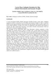
Figure 17: Bathymetry profiles for eight tracks shown on Figure 16.
As can be seen from Figure 16 and Figure 17 some of the paths cross the trench where water
depths up to 1000 m are found.
Two propagation codes were readily available for modelling the transmission of signals across
the trench. These were Kraken (Porter, 1994), a normal mode code, and RAM (Collins, 1993), a
parabolic equation code. These were run in the PC environment on a 500 MHz Pentium machine.
Each program was trialed with test, water and sediment parameters and found to give correct
results. The Kraken program is a "range independent" program, that is it can only be set up for a
single environment type of constant depth. Although the water column and seabed properties
could be expected to be reasonably constant throughout the study region (with water column
parameters primarily changing with depth) the bathymetry was not. Thus the RAM program was
chosen since it is "range dependant" or can deal with changing bathymetry, water column sound
speed profiles, or sediment characteristics. As a check the accuracy of the RAM and Kraken
programs were compared against each other. A constant environment problem was set up using
the seafloor parameters listed in Table 2, the water column sound speed profile shown in Figure
5 (or a 200 m deep Leeuwin current), a constant water depth of 450 m, a source at 40 m depth, a
receiver on the seabed at 450 m depth and a frequency of 24 Hz. The outputs of the two
programs over 5-10 km can be seen on Figure 18, along with an idealised case for ducted sound
or cylindrical spreading (10log10[range]).
The RAM and Kraken transmission loss curves shown on Figure 18 show identical trends, with
the small scale differences due to the different resolutions used in the calculations. Range steps
of 100 m were used in RAM and 250 m in the Kraken runs.
To visualise the 2D transmission loss field the Kraken output for the above run is presented on
Figure 19. It can be seen from this plot that regions of high and low transmission loss occur
scattered throughout the water column, and that as predicted by the ray plot of Figure 15, the loss
increases within the water column below the Leeuwin current base (200 m in the example)
beyond approximately 10 km. The 'patchiness' of the loss shown on Figure 19 is due to the
20