Molecular Phylogenetics & Evolution 65:974-994. - Dr. Sites ...

This article appeared in a journal published by Elsevier. The attached 

copy is furnished to the author for internal non-commercial research 

and education use, including for instruction at the authors institution 

and sharing with colleagues. 

Other uses, including reproduction and distribution, or selling or 

licensing copies, or posting to personal, institutional or third party 

websites are prohibited. 

In most cases authors are permitted to post their version of the 

article (e.g. in Word or Tex form) to their personal website or 

institutional repository. Authors requiring further information 

regarding Elsevier’s archiving and manuscript policies are 

encouraged to visit: 

http://www.elsevier.com/copyright

Author's personal copy 

Estimating divergence dates and evaluating dating methods using phylogenomic 

and mitochondrial data in squamate reptiles 

Daniel G. Mulcahy a,⇑ , Brice P. Noonan a , Travis Moss a , Ted M. Townsend b , Tod W. Reeder b , 

Jack W. Sites Jr. a , John J. Wiens c 

a Department of Biology, Brigham Young University, Provo, UT 84602, USA 

b Department of Biology, San Diego State University, San Diego, CA 92182-4614, USA 

c Department of Ecology and Evolution, Stony Brook University, Stony Brook, NY 11794-5245, USA 

article info 

Article history: 

Received 26 December 2011 

Revised 21 August 2012 

Accepted 22 August 2012 

Available online 7 September 2012 

Keywords: 

BEAST 

Lizards 

Penalized likelihood 

Phylogeny 

r8s 

Snakes 

1. Introduction 

abstract 

In recent years there has been increasing interest in using 

molecular-based phylogenies to infer the ages of clades (e.g., Sanderson, 

2002; Drummond et al., 2006; Rutschmann, 2006; Hedges 

and Kumar, 2009). Time-calibrated phylogenies have become integral 

to many evolutionary studies, including analyses of biogeography 

(e.g., Ree and Smith, 2008), species diversification (e.g., 

Ricklefs, 2007), and phenotypic evolution (e.g., O’Meara et al., 

2006). 

⇑ Corresponding author. Address: Laboratory of Analytical Biology, Smithsonian 

Institution, Museum Support Center, 4210 Silver Hill Road, Suitland, MD 20746, 

USA. Fax: +1 202 357 3043. 

E-mail address: MulcahyD@si.edu (D.G. Mulcahy). 

1055-7903/$ - see front matter Ó 2012 Elsevier Inc. All rights reserved. 

http://dx.doi.org/10.1016/j.ympev.2012.08.018 

Molecular Phylogenetics and Evolution 65 (2012) 974–991 

Contents lists available at SciVerse ScienceDirect 

Molecular Phylogenetics and Evolution 

journal homepage: www.elsevier.com/locate/ympev 

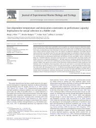
Recently, phylogenetics has expanded to routinely include estimation of clade ages in addition to their 

relationships. Various dating methods have been used, but their relative performance remains understudied. 

Here, we generate and assemble an extensive phylogenomic data set for squamate reptiles (lizards 

and snakes) and evaluate two widely used dating methods, penalized likelihood in r8s (r8s-PL) and 

Bayesian estimation with uncorrelated relaxed rates among lineages (BEAST). We obtained sequence data 

from 25 nuclear loci ( 500–1000 bp per gene; 19,020 bp total) for 64 squamate species and nine outgroup 

taxa, estimated the phylogeny, and estimated divergence dates using 14 fossil calibrations. We 

then evaluated how well each method approximated these dates using random subsets of the nuclear loci 

(2, 5, 10, 15, and 20; replicated 10 times each), and using 1 kb of the mitochondrial ND2 gene. We find 

that estimates from r8s-PL based on 2, 5, or 10 loci can differ considerably from those based on 25 loci 

(mean absolute value of differences between 2-locus and 25-locus estimates were 9.0 Myr). Estimates 

from BEAST are somewhat more consistent given limited sampling of loci (mean absolute value of differences 

between 2 and 25-locus estimates were 5.0 Myr). Most strikingly, age estimates using r8s-PL for 

ND2 were 68–82 Myr older (mean = 73.1) than those using 25 nuclear loci with r8s-PL. These results 

show that dates from r8s-PL with a limited number of loci (and especially mitochondrial data) can differ 

considerably from estimates derived from a large number of nuclear loci, whereas estimates from BEAST 

derived from fewer nuclear loci or mitochondrial data alone can be surprisingly similar to those from 

many nuclear loci. However, estimates from BEAST using relatively few loci and mitochondrial data could 

still show substantial deviations from the full data set (>50 Myr), suggesting the benefits of sampling 

many nuclear loci. Finally, we found that confidence intervals on ages from BEAST were not significantly 

different when sampling 2 vs. 25 loci, suggesting that adding loci decreased errors but did not increase 

confidence in those estimates. 

Ó 2012 Elsevier Inc. All rights reserved. 

Several methods for divergence-time estimation have been 

developed (e.g., Thorne et al., 1998; Yoder and Yang, 2000; Huelsenbeck 

et al., 2000; Sanderson, 2003; Thorne and Kishino, 2002; 

Drummond et al., 2006; Yang and Rannala, 2006; Lepage et al., 

2007; Rannala and Yang, 2007; Lartillot et al., 2009). The most 

widely used methods at present are based on ‘‘relaxed’’ molecular 

clocks where a general relationship between time and molecular 

divergence is assumed, and this relationship can vary across the 

tree. 

In the recent literature, two methods in particular have been 

widely used, penalized likelihood (implemented in r8s; Sanderson, 

2002, 2003) and Bayesian estimation with uncorrelated (‘‘relaxed’’) 

lognormally distributed rates among branches (implemented in 

BEAST; Drummond et al., 2006; Drummond and Rambaut, 2007). 

Penalized likelihood uses an input tree with branch lengths and assumes 

autocorrelation of rates among lineages, and the uneven-

ness (roughness) of the change in rates among lineages is penalized. 

A cross-validation method is used to find the optimal level 

of rate smoothing, and this ‘‘smoothing factor’’ defines the degree 

of autocorrelation. Using the Bayesian uncorrelated lognormal approach, 

rates of change are uncorrelated among branches and the 

rate on each branch is drawn from a lognormal distribution (Drummond 

et al., 2006; Drummond and Rambaut, 2007). For brevity, we 

hereafter use ‘‘r8s-PL’’ to refer to the penalized likelihood approach 

with r8s and ‘‘BEAST’’ to refer to the Bayesian uncorrelated lognormal 

method. However, we recognize that these software packages 

can be used to implement other approaches and that other software 

packages could potentially be used to implement these approaches. 

Many other methods for divergence-time estimation 

have also been frequently used, such as the Bayesian relaxed-clock 

method using autocorrelated rates among lineages (implemented 

in MultiDivTime; Thorne and Kishino, 2002). 

In addition to implementing the Bayesian uncorrelated approach, 

BEAST has other important advantages and is becoming 

widely used relative to r8s-PL and MultiDivTime. For example, 

BEAST can incorporate uncertainty in topology and branch lengths 

in estimating divergence dates and allows for different types of 

prior distributions (e.g., normal, uniform, and lognormal) on calibration 

points and other external sources (Drummond et al., 

2006; Drummond and Rambaut, 2007). Nevertheless, divergencetime 

estimates from r8s-PL remain common (e.g., Hugall et al., 

2007; Wiens, 2007; Burbrink and Pyron, 2008; Kozak et al., 2009; 

Spinks and Shaffer, 2009; Schulte and Moreno-Roark, 2010). Furthermore, 

because BEAST (and MultiDivTime) may not be practical 

on large data sets, r8s-PL may continue to be commonly used well 

into the foreseeable future. 

We know of no simulation studies that have directly compared 

divergence-date estimates from r8s-PL and BEAST. For example, a 

thorough simulation study by Battistuzzi et al. (2010) compared 

only BEAST and MultiDivTime. Further, although some previous 

empirical studies have estimated and compared dates from r8s 

and BEAST (e.g., Ribera et al., 2010; Wielstra et al., 2010), it is difficult 

to evaluate which method gives ‘‘better’’ or ‘‘worse’’ results 

without some non-arbitrary criterion. Only a few studies have attempted 

to systematically address differences in these methods 

with empirical data (Phillips, 2009; Egan and Doyle, 2010). 

In many ways, simulation studies offer the best way to evaluate 

these methods: one can generate a phylogeny with known dates 

and then examine how well each method estimates those dates, 

and under what conditions (e.g., Battistuzzi et al., 2010). However, 

there are many complications in estimating divergence dates from 

empirical data sets that may make fully realistic simulations challenging. 

For example, divergence-date estimation typically depends 

upon having one or more fossil calibration points (i.e., 

fossil taxa of ‘‘known’’ clade assignment and age), which tend to 

be available only sporadically among clades within a given group, 

but may strongly influence the estimated dates (e.g., Near and Sanderson, 

2004; Near et al., 2005; Rutschmann et al., 2007; Marshall, 

2008; Inoue et al., 2010). Further, different genes may be used to 

estimate dates, and these genes may differ not only in their length 

and rates of change, but also in their underlying histories (e.g., 

Maddison, 1997). This diverse array of complicated parameters 

may be difficult to simulate realistically. Thus, as a complement 

to simulation studies, it would be useful to also evaluate and compare 

dating methods using empirical data but with a non-arbitrary 

criterion to evaluate them. 

Additionally, divergence times are often estimated using a single 

locus (e.g., RAG-1; see Hugall et al., 2007; Wiens, 2007; Alfaro 

et al., 2009). Battistuzzi et al. (2010) demonstrated that Bayesian 

relaxed clock methods can produce more accurate estimates using 

multiple loci, but no similar studies have been conducted for r8s- 

PL. Empirical testing of the robustness of Bayesian dating methods 


D.G. Mulcahy et al. / Molecular Phylogenetics and Evolution 65 (2012) 974–991 975 

to sampling limited numbers of loci is still needed. It is also unclear 

how the use of more rapidly-evolving mitochondrial genes (in animals) 

may influence divergence dating relative to the use of more 

slowly-evolving nuclear loci. The impact of mitochondrial data 

may be particularly important in older clades, in which longer 

branches may be systematically overestimated by rapidly evolving 

mitochondrial genes (Zheng et al., 2011). 

In this paper, we take advantage of our phylogenomic studies of 

squamate reptiles (lizards and snakes) to evaluate and compare 

two widely used dating methods: r8s-PL and BEAST. We assemble 

a data set of 19,020 base-pairs (bp) from 25 protein-encoding nuclear 

loci for 64 ingroup taxa (representing major squamate clades 

and most families) and nine outgroup taxa, a data set considerably 

larger than those used in most dating studies. We then evaluate 

how well these methods approximate the estimated divergence 

dates based on all 25 loci, given random subsamples of a limited 

number of these loci (e.g., 2, 5, 10, 15, or 20 loci). Although we 

do not know what the true ages are for these clades, a method that 

gives highly variable estimates from a limited sample of loci may 

be problematic (i.e., two very different estimates for the same node 

cannot both be correct), relative to a method for which estimates 

from 2 or 5 loci are similar to those from 25 loci (even though this 

pattern does not guarantee that estimates from the latter method 

are actually correct). Additionally, it is important to understand 

how subsampling loci (i.e., using fewer loci) influences divergence-time 

estimates for these methods using empirical data. 

We also compare estimated divergence dates from the nuclear 

loci to those estimated from a single mitochondrial (mtDNA) gene. 

Although nuclear data are becoming increasingly accessible, many 

prominent analyses of phylogeny and divergence dates (in animals) 

continue to be based on mtDNA data alone (e.g., Santos 

et al., 2009; Schulte and Moreno-Roark, 2010). Few studies have 

systematically compared divergence dates estimated from mtDNA 

to those based on multiple nuclear loci (e.g., Wahlberg et al., 2009; 

Zheng et al., 2011) and our extensive sampling of nuclear loci provides 

an opportunity to address this issue. 

This is not the first study of phylogeny and divergence times in 

squamates. Recent studies have used molecular data to address 

higher-level squamate relationships (e.g., Townsend et al., 2004; 

Vidal and Hedges, 2005; Kumazawa, 2007; Wiens et al., 2010), 

and divergence dates (e.g., Vidal and Hedges, 2005; Wiens et al., 

2006; Hugall et al., 2007). Here, we provide the most extensive 

analysis of higher-level squamate phylogeny and divergence-time 

estimates to date, in terms of including many loci, taxa, and fossil 

calibration points. 

2. Materials and methods 

2.1. Taxonomic sampling 

Our taxon sampling was designed to address higher-level squamate 

phylogeny. We included at least two representatives of most 

families, except for some well-established clades (Anguimorpha, 

Iguania, Serpentes) for which we sampled fewer species. For outgroups, 

we used the tuatara (Sphenodon), the closest living relative 

to Squamata (e.g., Gauthier et al., 1988; Hugall et al., 2007), two 

crocodilians (Alligator and Crocodylus), two birds (Dromaius and 

Gallus), two turtles (Chelydra and Podocnemis), and two mammals 

(Homo and Mus). A list of sampled species, vouchers, and GenBank 

accession numbers is provided in Appendix A. 

2.2. Molecular sampling 

We obtained DNA sequence data from 25 protein-encoding nuclear 

loci. Some sequence data were used in our previous studies

on snakes (Wiens et al., 2008), iguanians (Townsend et al., 2011), 

and other squamates (Wiens et al., 2010); a total of 844 new sequences 

were generated for this study ( 20–30 new taxa per locus). 

Most loci were selected based on the protocol described by 

Townsend et al. (2008). This method allowed selection of gene regions 

that were: (1) single copy; (2) contained within a single 

exon; (3) short enough to amplify and sequence with a single pair 

of primers ( 500–1000 bp); and (4) variable enough to be informative 

among squamate families. Two additional loci were selected 

and sequenced based on their use in previous studies (RAG-1, 

Townsend et al., 2004; R35, Vidal and Hedges, 2005). 

To represent the mitochondrial genome, we used the proteinencoding 

gene NADH dehydrogenase subunit 2 (ND2), which is 

widely used in squamate phylogenetics (e.g., Macey et al., 2000; 

Townsend et al., 2004; Schulte and Moreno-Roark, 2010). Sequences 

were taken primarily from Townsend et al. (2004) as well 

as various other sources from GenBank. A few new ND2 sequences 

were also generated (all sources listed in Appendix A). We used 

only the portions of the sequences encoding the protein ND2 (i.e., 

tRNAs were not used because they are very short and difficult to 

align for the taxa in this study). 

For all samples, standard methods of DNA extraction, amplification, 

and sequencing were used. Primers for nuclear loci are listed 

in Appendix B. Sequence data were generated in the labs of J.W.S., 

T.W.R., and J.J.W. All sequences for a given gene were generated in 

the same lab, and the same individual was generally used for a given 

species across labs. Nucleotides for each gene were aligned by 

eye in MacClade (version 4.08; Maddison and Maddison, 2005) 

using amino acid translations. 

Preliminary parsimony analyses were conducted for each gene 

to detect possible contamination and other lab errors. When two 

species were identical or nearly identical, the gene was resequenced 

for one or both taxa. However, sequences were not 

excluded merely because they conflicted with previous taxonomy 

or with phylogenies from other genes. 

Some individuals were difficult to amplify and/or sequence for 

some loci. When this occurred, we designed new primers. However, 

we were still unable to amplify some loci for some taxa, 


976 D.G. Mulcahy et al. / Molecular Phylogenetics and Evolution 65 (2012) 974–991 

Table 1 

Number of taxa, characters, and best-fitting model of evolution for each locus and codon position. 

No. Taxa (73) Characters (19,020) Model 

Locus Missing Included Total Parsimony informative Constant Locus Position 1 Position 2 Position 3 

1 NTF3 2 71 516 311 158 GTR+I+C GTR+C GTR+C GTR+C 

2 SLC30A1 2 71 555 320 209 GTR+I+C HKY+I+C GTR+I+C GTR+I+C 

3 FSHR 3 70 753 345 345 GTR+I+C GTR+I+C GTR+I+C GTR+I+C 

4 ZEB2 0 73 885 326 485 HKY+I+C GTR+I+C GTR+I+C HKY+I+C 

5 MKL1 5 68 1047 621 317 GTR+I+C GTR+I+C GTR+I+C GTR+I+C 

6 TRAF6 0 73 651 379 217 SYM+I+C HKY+I+C GTR+I+C SYM+I+C 

7 PNN 7 66 1161 666 353 GTR+I+C GTR+C GTR+C GTR+I+C 

8 AHR 20 53 489 300 120 GTR+I+C HKY+C GTR+C HKY+I+C 

9 ECEL1 4 69 582 331 189 GTR+I+C GTR+C SYM+I+C GTR+C 

10 GPR37 13 60 507 219 279 GTR+I+C GTR+C GTR+I+C GTR+I+C 

11 PTGER4 10 63 468 201 240 HKY+I+C SYM+I+C GTR+I+C GTR+I+C 

12 NGFB 3 70 591 363 158 GTR+I+C GTR+I+C GTR+I+C GTR+C 

13 PTPN 16 57 690 479 143 HKY+I+C SYM+I+C GTR+I+C GTR+C 

14 ADNP 9 64 804 371 358 HKY+I+C K80+I+C GTR+C HKY+I+C 

15 BDNF 0 73 684 240 402 GTR+I+C GTR+C HKY+I+C GTR+I+C 

16 BMP2 10 63 642 307 283 GTR+I+C GTR+I+C HKY+I+C GTR+C 

17 DNAH3 4 69 663 326 298 GTR+I+C GTR+I+C GTR+I+C GTR+I+C 

18 FSTL5 6 67 621 275 274 HKY+I+C HKY+C GTR+I+C GTR+I+C 

19 RAG1 4 69 999 477 447 GTR+I+C GTR+I+C GTR+I+C GTR+I+C 

20 ZFP36L1 3 70 618 243 318 GTR+I+C GTR+I+C HKY+I+C GTR+C 

21 AKAP9 21 52 1461 963 298 GTR+I+C GTR+I+C GTR+I+C GTR+I+C 

22 SLC8A1 0 73 996 392 556 SYM+I+C HKY+I+C GTR+I+C GTR+I+C 

23 SLC8A3 4 69 1101 471 562 SYM+I+C GTR+I+C GTR+I+C GTR+I+C 

24 VCPIP1 5 68 801 333 428 SYM+I+C GTR+I+C GTR+I+C GTR+C 

25 R35 2 71 735 521 160 GTR+I+C SYM+I+C GTR+I+C GTR+I+C 

and these were coded as missing (‘‘?’’) in the combined analyses. 

The 25 genes ranged in completeness from 71% to 100% 

(mean = 91%; Table 1). Both simulation and empirical studies suggest 

that even extensive missing data need not prevent taxa from 

being accurately placed in phylogenetic analyses, especially if the 

overall number of characters is large (e.g., Wiens, 2003; Driskell 

et al., 2004; Philippe et al., 2004; Wiens et al., 2005; Wiens and 

Moen, 2008; Wiens and Morrill, 2011). Furthermore, limited analyses 

suggest that branch-length estimation need not be adversely 

affected by missing data, especially if rate heterogeneity among 

genes is accounted for by partitions (Wiens and Morrill, 2011). 

2.3. Phylogenetic analyses 

Phylogenetic analyses were conducted on the entire 25-locus 

data set using maximum parsimony (MP) with PAUP (v4.0b10; 

Swofford, 2002), maximum likelihood (ML) with RAxML (v7.0.4; 

Stamatakis et al., 2008), and Bayesian inference using MrBayes 

(v3.1.2; Huelsenbeck and Ronquist, 2001). Parsimony analyses 

were conducted using the heuristic search option, with 100 

random taxon-addition sequence replicates, tree-bisectionreconnection 

branch swapping, and no limit on the number of 

shortest trees retained. Gaps (i.e., indels) were treated as missing 

data for all three methods. Non-parametric bootstrap analyses 

were conducted with 1000 pseudoreplicates using the same 

heuristic search options but with 25 random, stepwise-addition 

replicates per bootstrap replicate. Nodes with bootstrap values 

P70% were considered strongly supported (Hillis and Bull, 1993; 

but see their caveats). 

For the Bayesian analyses, MrModeltest (v2.3; Nylander, 2004) 

was used to estimate the best-fit model for each partition, using 

the Akaike Information Criteria (Posada and Buckley, 2004). We 

tested each gene separately, and each codon position within each 

gene (Table 1). Bayesian analyses were conducted with three partitioning 

strategies, and Bayes factors (BF; Kass and Raftery, 1995) 

were used to select the optimal partitioning strategy. Comparison 

between Bayes factors was evaluated as: 2ln (BF12), where BF12 

represents the difference between the estimated mean marginal

likelihoods of the two partitioning strategies (from the harmonic 

mean of the log likelihoods of the post-burn-in trees from each 

analysis, see below). A difference in Bayes factors >10 was considered 

to significantly support the alternative strategy (e.g., Kass and 

Raftery, 1995; Nylander et al., 2004; Brandley et al., 2005). The first 

partitioning strategy consisted of a separate partition for each codon 

position across all genes (three partitions total), the second 

consisted of one partition per gene (25 partitions total), and the 

third consisted of a partition for each codon position for each gene 

(75 partitions). Each Bayesian analysis was initially run twice for 

10 10 6 generations, saving trees every 1000 generations, with 

four chains (default temperatures), and model parameters unlinked 

between partitions. Convergence of runs was determined 

by comparing the average standard deviation of split frequencies 

(ASDSF) in MrBayes and by plotting log likelihoods (lnL) against 

number of generations in Tracer (v1.4; Rambaut and Drummond, 

2007). Trees generated prior to reaching convergence were discarded 

as burn-in. The best-fitting partitioning strategy (75 partitions) 

was subsequently run in MrBayes for 80 10 6 generations 

(with other settings as before). Estimated posterior probabilities 

(Pp) for each clade were taken from a 50% all-compatible, majority-rule 

consensus of post-burn-in trees. Clades with Pp P 0.95 

were considered strongly supported (e.g., Alfaro et al., 2003; Huelsenbeck 

and Rannala, 2004). 

For the ML analysis, we used the rapid hill-climbing algorithm 

in RAxML (VI-HPC 7.0.4; Stamatakis et al., 2008) and the GTR+I+C 

model option for 100 inferences to determine the optimal likelihood 

tree with 75 partitions (see above). The GTR model is the only 

substitution model implemented in RAxML, and our model-testing 

analyses suggest that this model has the best fit for the majority of 

genes and partitions (Table 1). We used the standard 25 discrete 

GAMMA rate categories. A bootstrap analysis was conducted with 

1000 replicates, and clades with support P70% were considered 

strongly supported (e.g., Wilcox et al., 2002). 


Table 2 

Fossil calibration points used for estimating dates of divergence (nodes in Fig. 1). For BEAST-mix, nodes with a range of minimum and maximum ages were implemented with 

normal priors, whereas those with minimum-only constraints were implemented with lognormal priors. Dates for stages are from Gradstein et al. (2004). See Appendix C for 

detailed description of each calibration point. HPrD = Highest Prior Densities calculated in BEAUTi for use in BEAST. 

Node 

Fig. 1 

Date (Myr) 95% HPrD (median, 

upper and lower 

limits) 

Fossil calibration Age (period/stage) Reference and comments 

1 312.3–330.4 321.3 (313.7–328.9) Reptile–mammal split Late Carboniferous Benton and Donoghue (2006) 

2 255.9–299.8 277.8 (259.4–296.2) Lepidosauria–Archosauria Permian Donoghue and Benton (2007) and Benton et al. 

(2009) 

3 222.8 (min) 223.4 (222.9–225.9) Oldest rhynchocephalian Triassic Sues and Olsen (1990) and Evans (2003) 

4 239–250.4 244.7 (239.9–249.5) Bird–crocodile Triassic Benton et al. (2009) 

5 54 (min) 54.51 (54.1–57.1) Gekkotan Yantarogekko Lower Eocene Bauer et al. (2005) 

6 65.2 (min) 65.81 (65.3–68.3) Konkasaurus Maastrichtian (Late 

Cretaceous) 

Krause et al. (2003) 

7 70.0 (min) 70.61 (70.1–73.1) Chamops, Haptosphenus, 

Letpochamops, 

Meniscognathus 


Campanian (Late Cretaceous) Estes (1964), Bryant (1989) and Denton and 

O’Neill (1995) 

8 111 (min) 111.5 (111.1–114.1) Hodzhakulia Aptian–Albian (Early 

Cretaceous) 

Evans (2003) and Wiens et al. (2006) a 

9 92.7 (min) 93.31 (92.8–95.8) Coniophis Cenomanian (Late Cretaceous) Marsh (1892) 

10 70.0 (min) 70.61 (70.1–73.1) Palaeosaniwa, Telmasaurus Campanian (Late Cretaceous) Bryant (1989), Borsuk-Bialynicka (1984) and 

Cherminotus 

Gao and Norell (2000) 

11 70.0 (min) 70.61 (70.1–73.1) Odaxosaurus Campanian (Late Cretaceous) Bryant (1989), Wiens et al. (2006) a , Hugall 

et al. (2007) and Conrad (2008) 

12 70.0 (min) 70.61 (70.1–73.1) Priscagamines, iguanines, Campanian–Maastrichtian Gao and Norell (2000) and Conrad (2008) 

and Isodontosaurus (see 

text) 

(Late Cretaceous) 

13 99.6 (min) 100.2 (99.7–102.7) Primaderma Albian–Cenomanian (Late Nydam (2000), Vidal and Hedges (2005) 

Cretaceous) 

a , 

Wiens et al. (2006) a , Hugall et al. (2007) a and 

Conrad (2008) 

14 70.0 (min) 70.61 (70.1–73.1) Contogenys, Sauriscus Campanian (Late Cretaceous) Estes (1969), Bryant (1989) 

a Previous studies that used these fossil calibrations, though exact dates chosen varied (see text). 

2.4. Calibrating divergence times 

We first estimated clade ages for both methods using all 25 loci 

and 14 fossil calibration points. We used the oldest known fossil 

taxon confidently placed within the crown group of a clade to 

establish a minimum age for the most recent common ancestor 

of that clade. Some fossil taxa are assigned to modern families or 

other clades but cannot be confidently assigned to the modern 

crown group; in these cases, we used that fossil taxon to determine 

the minimum age of the stem group for the clade instead (i.e., the 

node immediately below the crown group). Fossil taxa were used 

that could be confidently assigned to clades based on recent phylogenetic 

analyses (e.g., Conrad, 2008; Wiens et al., 2010), and following 

proposed taxonomy in the Paleobiology Database (PBDB: 

http://paleodb.org). We used the most recent, comprehensive 

assessment of ages for geological strata to obtain dates for each 

fossil used (Gradstein et al., 2004) or the PBDB for strata not listed 

in Gradstein et al. (2004). We used the minimum age of the stratum 

as a minimum calibration age for the crown group of the relevant 

clade. When error terms were given for a stratum, we used 

the minimum age minus the error. 

To find calibration constraints within squamates, we performed 

a thorough review of the paleontological literature, starting with 

fossil calibrations used in previous dating analyses (e.g., Vidal 

and Hedges, 2005; Wiens et al., 2006; Hugall et al., 2007). Because 

these studies used different dating methods, taxon sampling, and 

criteria for assigning calibrations points, only three calibration 

points within Squamata were shared between these studies and 

ours (Table 2). 

The age of a given fossil can be used to set the minimum age of a 

given clade (Drummond et al., 2006), but determining the maximum 

age of a clade is more difficult, because a clade may be older 

than the earliest known fossil (e.g., Benton and Donoghue, 2006). 

However, previous studies have determined minimum and

maximum age constraints for three of the outgroup clades used 

here (e.g., Müller and Reisz, 2005; Benton and Donoghue, 2006; 

Benton et al., 2009). In total, we utilized 10 minimum age 

constraints within Squamata, including nearly every major 

clade (e.g., Evans, 2003), and four among the outgroup taxa (three 

minimum–maximum, one minimum only; Table 2). We provide 

full details and justification for each calibration point, and discuss 

differences in calibration choices between previous studies and 

ours, in Appendix C. 

2.4.1. Evaluating dating methods 

Our comparisons of dating methods focused on the ages of seven 

‘‘focal’’ nodes that were recovered in all of our phylogenetic 

analyses (labeled A–G; Fig. 1). However, we also explored the differences 

between methods across all nodes, to see if the observed 

effects were consistent throughout the tree. We first estimated 

ages using the entire data set (25-locus) with the ML topology in 

r8s-PL and BEAST. The program r8s requires an input tree with 

branch lengths, whereas BEAST can estimate phylogeny and divergence 

dates simultaneously. However, to be consistent, we used 



the optimal topology from our ML analysis as the input tree for 

both methods (note that any potential uncertainty in topology 

should have little impact on estimated ages, given the strong support 

for most nodes; see Section 3). 

For the subsampling analyses, a random number generator 

(http://www.random.org/) was used to select a set of loci for each 

replicate (or ‘‘pseudoreplicate’’). Loci were sampled without 

replacement, such that no locus was represented twice in a given 

data set. Ten replicate data sets were generated for each level of 

sampling (2, 5, 10, 15, and 20 loci). Loci were then concatenated, 

and each data set was analyzed in r8s-PL and BEAST as described 

below. In theory, we could have included analyses based on a single 

locus, but this would have been potentially problematic given 

the short length of some sequences ( 500 bp) and because we 

were missing data for some loci for all members of a particular 

clade (e.g., Dibamidae; Table 1). Although it may seem problematic 

that we only used 10 replicates for each level of sampling, the 

BEAST analyses were extremely computationally intensive, with 

many replicates each requiring >14 days on a supercomputer 

(see below). 

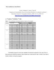
Fig. 1. Maximum likelihood phylogram for squamate reptiles based on 25 nuclear loci (19,020 bp). Bootstrap values are shown only for nodes that received values less than 

100%. Nodes with numbered circles (1–14) represent those with calibrations based on fossil data (see Table 2). Square nodes with letters (A–G) indicate focal nodes for 

comparison of estimated divergence dates in the subsampling analyses. The terminal ‘‘Gymn.’’ identifies the clade Gymnophthalmidae.

Data sets ranged in size based on the number of loci from 1137 

to 1932 bp, mean = 1449.3 bp (2-locus); 3075–4731, 3763.8 

(5-locus); 6375–8595, 7597.8 (10-locus); 11,052–12,561, 11626.2 

(15-locus); and 14,157–16,167, 15126.3 (20-locus). The loci in 

each data set and size of each are given in Appendix D. 

2.4.2. Mitochondrial data 

We obtained published sequences of ND2 for 51 of the 73 species 

in the nuclear data set, generated new ND2 data for six species, 

used closely related species in GenBank for 15, and we were unable 

to obtain suitable data or a replacement for one taxon (see below). 

For 10 of these replacements, we used mtDNA data from the same 

genus but a different species, relative to the nuclear data set. For 

the five others, we used closely related genera, as determined from 

previous phylogenetic studies (Pelomedusa for Podocnemis, Krenz 

et al., 2005; Python–Aspidites, Wiens et al., 2008; Sphaerodactylus–Gonatodes, 

Gamble et al., 2008; Leposoma–Colobosaurus, Castoe 

et al., 2004; and Chalcides–Amphiglossus, Brandley et al., 2005). For 

Callopistes, we were unable to obtain a suitable representative for 

ND2, and this taxon was excluded in the ND2 data set. In total, sequences 

for 66 taxa were downloaded from GenBank and we collected 

new data for six (see Appendix A). The use of these 

alternative taxa should have little impact on branch length estimates 

at these higher taxonomic levels, and it allowed us to use 

the same calibration points as for the nuclear data. The ND2 alignment 

is 1044 bp in length, with 878 parsimony-informative characters. 

Overall, the sampling of characters and taxa was similar 

between the ND2 and 2-locus data sets, even though ND2 was considerably 

more variable. 

2.4.3. Estimating divergence dates in r8s 

We used cross-validation to find the best smoothing factor for 

our entire data set (25-locus) and for each replicate data set (locus 

subsampling) using the optimal ML inferred topology. For each 

data set, we started the cross-validation process with a log10 value 

of -1, increasing by increments of 0.1, with 100 estimates total. 

Then, we fine-tuned the smoothing values by selecting the optimal 

value (lowest Chi-square value) based on the 0.1 increments and 

performed additional cross-validation within the local range of 

the first optimal value using 100 increments of 0.01 each, until 

the lowest Chi-square value was obtained, yielding the final optimal 

smoothing value. 

We used the penalized likelihood method in r8s, using the truncated 

Newton algorithm and the additive penalty function. We also 

tested the logarithmic penalty function on the 25-locus data set. 

However, the additive function is thought to be more appropriate 

when root nodes are calibrated (Sanderson, 2002); therefore, we 

used the additive function for the iterations of varying numbers 

of loci. Both methods gave very similar age estimates for our data 

(see Section 3), suggesting that use of the additive vs. logarithmic 

function should have little impact on our conclusions. 

Pruning the farthest outgroup prior to analyses is recommended, 

because of the problem of where to distribute the branch 

lengths between the root and remaining taxa (Sanderson, 2004). 

However, to avoid discarding our oldest calibration (mammal– 

reptile), which would compromise comparisons with the BEAST results, 

we included the mammal–reptile node and distributed the 

branch lengths using mid-point rooting in FigTree (v1.2.3, Rambaut, 

2009). Preliminary analyses with the root outgroup removed 

(and consequently the mammal–reptile calibration removed) estimated 

dates even older than with them included (suggesting that 

the older age estimates from r8s-PL relative to BEAST are not an 

artifact of including the root in r8s-PL; see Section 3). Therefore, 

we ran our 25-locus data set in r8s-PL with our optimal ML topology, 

with all 14 calibration points (calibrations 1–2, 4 with mini- 



mum and maximum values, and calibrations 3 and 5–14 with 

minimum values only; see Table 2). 

To approximate bootstrap confidence intervals on dates for the 

seven nodes in the 25-locus data set, we created 1000 bootstrap 

replicates of the 25-locus data set using ‘seqboot’ in Phylip 

(v3.68; Felsenstein, 2004), and estimated branch lengths for each 

bootstrap-replicated data set on the optimal ML topology using 

RAxML. We determined the smoothing factor for each tree (using 

cross-validation, see above), and estimated confidence intervals 

for each node using the r8s bootstrap kit (Eriksson, 2007), with corrections 

suggested by Burbrink and Pyron (2008), and reported results 

of the approximate bootstrap confidence quadratic (ABCq) 

method. 

All subsampling analyses, as well as the separate mtDNA analysis, 

were done with branch lengths estimated in RAxML using 

the GTR+I+C model, partitioned by codon separately for each locus. 

In four of the subsampled data sets (three of the 2-locus, and one of 

the 5-locus), a zero-length branch was estimated for one of the 

calibration nodes (either node 2 or 12), and these nodes were excluded 

from those four replicates. Also, in three cases for the 

2-locus data sets, 1–3 taxa lacked data for both sampled loci and 

were excluded from those analyses (see Appendix D for details 

on both of these exceptions). Although confidence intervals for 

each node for each subsampling replicate might be useful in theory, 

these would have been very difficult to estimate (e.g., each 

of the 10 replicates would each require 100 replicates). 

2.4.4. Estimating divergence dates in BEAST 

For all analyses in BEAST we used the same fixed topology (ML) 

used in r8s-PL. Each codon position in each gene was assigned a 

separate partition, based on the results of the comparisons of partitioning 

strategies described above. We used the GTR+I+C model 

for all partitions for the entire data set and each subsampling analysis, 

as this model was selected for most partitions in our phylogenetic 

analyses (Table 1). We used the uncorrelated lognormal 

relaxed-clock method with a Yule speciation process for all analyses. 

For three calibration nodes for which we had minimum and 

maximum values (nodes 1–2 and 4; Fig. 1), we used a normal prior 

with a mean value at the midpoint between the minimum and 

maximum values (node 1 = 321.3, node 2 = 277.8, node 

4 = 244.7). We also chose standard deviation (stdev) values such 

that the upper and lower limits of the 95% HPrD (Highest Prior 

Densities) intervals correspond to the minimum and maximum 

estimated ages based on the fossil record (Table 2; i.e., node 1 

stdev = 4.64; node 2 = 11.2; node 4 = 2.9). For all other nodes (minimum 

values only) we used the lognormal prior, set the mean to 

1.0, stdev to 1.0, and used offset values equal to the minimum calibration 

ages (i.e., for Calibration 3, offset = 222.8; see Table 2 for 

HPrD values). We acknowledge that this value for the mean is arbitrary 

and somewhat low, such that the range of HPrD values are 

relatively narrow, but we note that the HPrD is only for the prior 

and does not necessarily determine the final estimated dates. In 

theory, narrower HPrDs may contribute to age estimates from 

BEAST analyses being younger than those from r8s-PL (see Section 

3), but this does not appear to explain the differences in 

robustness of these methods to sampling few loci (based on an 

analysis using different types of calibration priors, see below). Because 

we employed two types of calibration priors in these analyses 

(minimum and minimum + maximum), we refer to analyses 

run with the above calibration scheme as ‘‘BEAST-mix.’’ 

We also tested whether the differences in estimated ages that 

we observed between r8s-PL and BEAST-mix (see Section 3) might 

be related to how these methods treat fossil calibration points. We 

performed an analysis of our 25-locus data set using uniform distribution 

priors on all calibrations in BEAST (referred to as the 

‘‘BEAST-uniform’’ analysis hereafter), using the same minimum

age for each clade used in r8s-PL. The uniform prior is similar to the 

calibration method implemented in r8s. For the BEAST-uniform 

analyses, we set a maximum value (222.7, min. age for Lepidosauria) 

for all nodes within Squamata to avoid incompatible estimates 

(i.e., when maximum values were set to infinity, the program 

unexpectedly quit, seemingly because estimates for shallow clades 

were sometimes older than calibrations for deeper clades). Additionally, 

we ran the BEAST-uniform calibration scheme on all 10 

of the 2-locus data sets to see if the results would be similar to 

those from the BEAST-mix analyses or instead show greater variability 

in estimated dates with a smaller number of loci (similar 

to r8s-PL). 

We also ran BEAST without our sequence data in order to sample 

only the prior distribution (referred to as the ‘‘BEAST-prior’’ 

analysis hereafter). This was performed using the BEAST-mix calibration 

scheme to determine if the calibration priors alone determined 

the estimated dates, or if the estimates are strongly 

influenced by the sequence data (e.g., Drummond et al., 2006). Estimates 

from the BEAST-prior analysis were markedly different from 

those with sequence data (Appendix E), especially for nodes other 

than the 14 calibration nodes. As expected, point estimates on fossil-calibrated 

nodes (1–14) were much closer (range of absolute 

values for differences between the estimates for these nodes is 

0.1–19.3; mean = 5.1 Mya) than those from nodes lacking fossil 

calibration priors (range = 0.6–56.1; mean = 15.8 Mya). Overall, 

these analyses indicate that our BEAST results are determined by 

the combination of the sequence data and the priors, and not by 

the priors alone (see Section 3 for a comparison of the width of 

the 95% Highest Posterior Densities [HPDs] for estimates with 

and without sequence data). 

For BEAST analyses of the 25-locus data set, we aimed to 

achieve ESS (effective sample size) values >200 for the estimated 

ages for the seven focal nodes (A–G). However, we were not able 

to achieve these desired values, even after using several strategies. 

These strategies included (a) changing the number of partitions (3 

vs. 75), (b) runs ranging from 100 to 300 10 6 generations (sampling 

every 1000–10,000 generations), and (c) combining six analyses 

(each run for 500 10 6 generations sampling every 10,000), 

and one analysis run for 1 10 9 (1 billion) generations, sampling 



Table 3 

Clade ages estimated by r8s-PL for the seven focal nodes, including estimates for all 25 loci (including lower and upper 95% bootstrap confidence intervals, LCI and UCI), mean 

estimates from subsampling experiments, mean absolute value of differences from 25-locus estimates in parentheses, and estimated values from a single mitochondrial gene 

(ND2). 

Node: 25-Locus LCI UCI 2-Locus 5-Locus 10-Locus 15-Locus 20-Locus ND2 

A 191.8 186.38 194.2 195.2 (12.6) 191.4 (6.6) 194.3 (3.6) 192.5 (2.5) 192.0 (2.0) 264.6 

B 189.5 183.7 191.6 193.9 (11.6) 190.0 (6.7) 192.0 (3.6) 190.5 (4.1) 189.6 (2.0) – 

C 184.6 179.1 186.8 186.4 (11.1) 184.8 (5.8) 186.9 (3.1) 185.5 (2.2) 185.0 (1.8) 262.7 

D 174.0 169.8 176.6 176.8 (11.1) 173.0 (5.4) 176.2 (2.7) 174.6 (1.9) 174.3 (1.4) 261.6 

E 167.9 161.2 171.9 167.7 (9.3) 168.8 (5.6) 169.8 (3.4) 168.9 (2.5) 168.4 (1.8) 243.3 

F 163.9 159.0 167.5 169.0 (11.9) 162.4 (7.3) 165.9 (2.3) 164.6 (1.7) 163.9 (1.3) 239.7 

G 169.8 165.8 172.3 169.3 (8.6) 168.3 (5.2) 172.0 (3.0) 170.3 (1.9) 170.1 (1.3) – 

Table 4 

Clade ages estimated by BEAST-mix for the seven focal nodes, including estimates for all 25 loci (including effective sample size, ESS, and lower and upper 95% credibility 

intervals, LCI and UCI), mean estimates from subsampling experiments, mean absolute value of differences from 25-locus estimates in parentheses, and estimated values from a 

single mitochondrial gene (ND2). The overall posterior value and log likelihood ( lnL) scores are shown on the bottom rows for the 25 loci and ND2, ESS values for 25 loci. 

Node: 25-Locus ESS LCI UCI 2-Locus 5-Locus 10-Locus 15-Locus 20-Locus ND2 

A 180.0 82.3 160.2 197.9 181.8 (3.8) 181.1 (1.8) 180.9 (2.5) 180.4 (1.8) 181.0 (1.6) 175.9 

B 173.4 83.4 154.4 190.5 173.3 (2.9) 174.1 (2.3) 174.7 (1.6) 174.5 (1.6) 174.3 (1.5) 171.3 

C 162.8 68.1 145.4 179.9 162.5 (3.4) 164.4 (2.1) 163.7 (1.6) 163.4 (1.3) 163.5 (1.3) 165.1 

D 149.1 64.7 135.3 164.6 149.5 (3.5) 149.8 (2.2) 149.7 (1.4) 149.7 (1.4) 149.5 (1.4) 158.6 

E 123.3 56.8 92.1 155.0 118.8 (7.9) 122.4 (5.1) 121.4 (5.1) 124.7 (3.3) 122.4 (3.7) 117.2 

F 135.0 86.9 120.3 150.2 137.0 (3.9) 135.4 (2.4) 135.5 (1.8) 135.7 (1.5) 135.4 (1.1) 139.7 

G 140.8 63.8 127.0 156.5 141.9 (3.7) 140.7 (2.0) 141.5 (1.5) 141.4 (1.4) 140.9 (1.3) 155.8 

Posterior 303275.3 308.9 – – – – – – – 51531.5 

lnL 303329.5 24649.9 – – – – – – – 799.9 

every 100,000 (more frequent sampling produced file sizes >1 GB 

that were not readable in Tracer). We found that overall posterior 

values for some runs (of the same date file) reached stationarity by 

20 10 6 generations, whereas others took nearly 450 10 6 generations, 

and some runs appeared to reach stationarity but never 

achieved overall posterior scores (e.g., 303,355) equivalent to 

other runs with better posterior scores. Therefore, we used Log- 

Combiner (in BEAST) to combine analyses utilizing the same partitioning 

strategy (75 partitions) that reached similar overall 

posterior values ( 303,272 to 303,281), to obtain the highest 

ESS values possible for the ages of the focal nodes (A–G). In the 

end, we combined six runs (100 10 6 , 200 10 6 , 300 10 6 ,2at 

500 10 6 , and 1 at 1 10 9 ) with a post-burn-in (separately for 

each run) log file with 675 10 6 states. We report these values 

and associated dates as our best estimates for BEAST and for comparison 

with the subsampling analyses. Although some readers 

might be concerned that we did not achieve the desired ESS values 

with 25 loci, our results show that our 10 replicates of 2- and 5-loci 

(which all achieved ESS values >200) each yielded similar estimated 

ages for all focal nodes as the replicates with 10-, 15-, 20-, 

and 25-loci (which had ESS values 200 for ages for nodes A–G for ND2, 2-locus, and some 

5-locus runs. However, for the other 5-locus and all 10-, 15-, and 

20-locus data sets, we ran analyses for 500 10 6 generations, sampling 

every 10,000 generations. The ESS values for estimates on 

nodes A–G ranged from 328 to 1690 (mean = 702) for the 2-locus 

analyses, but ranged from 100 to 448 (mean = 173) for the 5-locus 

analyses, and became progressively lower as more loci were added 

(see results from 25-locus analyses, Table 4). 

The ESS values improved for the 5-locus analyses when we increased 

the number of generations to 500 million. Therefore, ESS 

values greater than 200 might be possible for all analyses if it were 

feasible to run them for more generations. However, as explained

above, we ran one analysis of the 25-locus data set for 1 billion 

generations, which exceeded our allowed time on the supercomputer, 

and still did not achieve ESS values > 200. 

2.5. Autocorrelation of rates 

Recent simulations (Battistuzzi et al., 2010) suggest that the relative 

accuracy of dating methods for a given data set may hinge on 

whether the underlying rates of molecular evolution are phylogenetically 

autocorrelated (assumed by r8s and MultiDivTime) or 

uncorrelated (BEAST). We assessed autocorrelation in our 25-locus 

data set using two methods. First, we used BEAST and examined 



the covariance statistic in Tracer (Drummond et al., 2006). If the 

95% HPD for the covariance statistic contains zero, then there is 

no evidence for autocorrelation. However, this method has been 

criticized for its lack of power to detect autocorrelation in simulations 

(Battistuzzi et al., 2010). Therefore, we also assessed autocorrelation 

by comparing the natural logs of Bayes factors (lnBF), 

estimated using thermodynamic integration between the default 

‘‘deconstrained’’ model and both ‘‘lognormal’’ (autocorrelated) 

and ‘‘uncorrelated gamma’’ clock models (Lepage et al., 2007), with 

the number of integration steps (K) = 10,000, saving every 10 

points. These latter analyses were conducted in PhyloBayes 

(v3.2e, Lartillot et al., 2009). 

Fig. 2. Chronogram for squamate reptiles estimated by r8s-PL based on 25 nuclear loci (scale on x-axis in Mya). Scale bars around nodes (identified in Fig. 1) indicate the 95% 

ABCq upper and lower bootstrap confidence intervals (values are listed in Table 3). Inset shows types of calibrations used for particular nodes; probabilities increase along 

y-axes and ages decrease on x-axes. The minimum–maximum calibration estimates have a uniform probability for any age between the minimum and maximum calibration 

points, and the minimum only calibration estimates have uniform probability for any age between the minimum and the next calibration deeper in the tree (similar to the 

‘‘uniform’’ prior in BEAST).

2.6. Computational hardware 

Analyses using PAUP and r8s-PL were conducted on standard 

MAC OSX desktop computers. MrBayes and RAxML analyses were 

conducted on the BYU Life Sciences Computational Cluster, which 

consists of 68 nodes running Debian Linux, each node with two Intel 

Xeon quad core processors (E5345) at 2.33 GHz with 16 GB of 

RAM, a 250 GB hard drive and Mellanox 4x Infiniband card providing 

20 Gb connectivity between nodes. BEAST analyses were run in 

the Fulton Supercomputing Lab (BYU) on marylou5, a Linux cluster 

of 320 nodes (2560 CPUs, 7680 GB total memory). BEAST analyses 

were run using eight processors per node and took on average from 



8 to 10 days, and the maximum (1 10 9 generations) taking 

26 days, exceeding the default time allowed by 10 days. 

3. Results 

3.1. Phylogenetic analyses 

The phylogenies estimated for all 25 loci (19,020 bp; 9780 parsimony-informative 

characters) from the ML (Fig. 1), MP, and 

Bayesian analyses are generally similar to each other (Supplementary 

materials, Figs. S1 and S2, respectively). These phylogenies are 

Fig. 3. Chronogram for squamate reptiles estimated by BEAST-mix based on 25 nuclear loci (scale on x-axis in Mya). Scale bars around nodes indicate the 95% credibility 

intervals (values for nodes A–G are listed in Table 4). Inset shows types of calibrations used for particular nodes; probabilities increase along y-axes and ages decrease on 

x-axes. The normal prior for clade age was used for clades with both minimum and maximum calibration ages, and has the highest probability around the midpoint between 

the minimum and maximum. The lognormal distribution on the prior for clade ages is used for clades with a minimum calibration point, and has the highest probability close 

to the minimum age.

also similar to those from other recent molecular analyses of higher-level 

squamate relationships (e.g., Townsend et al., 2004; Vidal 

and Hedges, 2005; Wiens et al., 2010). All of our analyses placed 

Dibamidae as sister to all other squamates, with moderate to 

strong support (MP and ML bootstrap = 98% and 72%, respectively; 

Bayesian Pp = 0.93). Although all of our analyses found Toxicofera 

(Anguimorpha, Iguania, Serpentes) to be well supported, relationships 

among the three major clades within this group were not. 

Relationships within Toxicofera varied among methods, with ((Iguania 

+ Serpentes) Anguimorpha) supported in our MP analysis and 

((Iguania + Anguimorpha) Serpentes) supported in our ML and 

Bayesian analyses. The only other differences between analyses 

(MP, Bayesian, and ML) within Squamata involved relationships 

within Scincidae. The MP tree shares 65 of 70 nodes with the ML 

and Bayesian trees (normalized consensus fork index = 0.929; symmetric-difference 

distances = 10) whereas the ML and Bayesian 

trees share 67 of 70 nodes (normalized consensus fork index 

= 0.957; symmetric-difference distance = 6). 

3.2. Estimating dates of divergence 

Clade ages based on 25 loci in r8s-PL (Fig. 2; Table 3) and 

BEAST-mix (Fig. 3; Table 4) are generally similar to those in other 

studies (e.g., Vidal and Hedges, 2005; Wiens et al., 2006; Hugall 

et al., 2007; see Table 5 for explicit comparisons). However, nodes 

A–G are consistently estimated as older by r8s-PL relative to 

BEAST-mix (11.8–44.6 Myr older, mean 25.3 Myr; Fig. 4; Tables 3 

and 4). This trend is generally consistent across the tree, but varies 

across different clades (Figs. 5 and 6). Although estimates from r8s- 

PL are much older for some nodes deeper in the tree (e.g., Lepidosauria) 

and at the tips (e.g., Gekko–Phelsuma), this varies somewhat 

from group to group (e.g., estimates are nearly the same within 

snakes, but markedly different within other clades such as geckos, 

scincids, and iguanians; Fig. 5). Results from r8s-PL with the logarithmic 

penalty function are not significantly different from those 

with the additive function (mean difference = 1.4 Myr, d.f. = 69, 

t-value is 1.686, and P = 0.096; Supplementary materials Fig. S3). 


Analyses using BEAST-mix and PhyloBayes both suggest that 

rates are uncorrelated and not autocorrelated, respectively, indicating 

that the model assumed by BEAST-mix may fit these data 

better than the model assumed by r8s-PL. The 95% HPD values 

for the covariance statistic on our combined log file for BEASTmix 

contained zero (mean = 0.0211; HPD lower = 0.149, 

upper = 0.1142; ESS = 214.588), suggesting a lack of autocorrelation 

among rates (Drummond et al., 2006). Further, analyses using 

PhyloBayes for the lognormal (autocorrelated) model gives 

lnBF = 7.3982 (interval = 10.9694 to 8.84922) and for the 

uncorrelated gamma model lnBF = 10.1284 (interval = 9.92258– 

13.0388). The lognormal interval contains negative values, indicat- 



Table 5 

Comparison of squamate divergence dates estimated here to those from previous studies. Confidence intervals (95%) for previous studies are shown where available. The methods 

used by various authors are shown below the reference. 

Node Vidal and Hedges (2005) Wiens et al. (2006) Hugall et al. (2007) This study This study 

MultiDivTime r8s–PL r8s–PL r8s–PL BEAST-mix 

A 240 (251–221) 178.7 (184–173) – 191.8 (186–194) 180.0 (160–198) 

B 225 (240–207) – 190 (204–176) 189.5 (184–192) 173.4 (154–191) 

C 215 (230–199) 173.9 (179–169) 176 (190–162) 184.6 (179–187) 162.8 (145–180) 

D 191 (206–179) 168.3 (174–163) – 174.0 (170–177) 149.1 (135–165) 

E 192 (209–176) 157.6 (167–149) 162 (175–149) 167.9 (161–172) 123.3 (92–155) 

F 177 (193–164) 161.6 (168–156) – 163.9 (159–167) 135.0 (120–150) 

G 178 (194–167) 163.9 (169–158) 158 (171–145) 169.8 (166–172) 140.8 (127–157) 

ing that it often performed worse than the unconstrained model 

(Lepage et al., 2007). 

3.4. Comparison of dating methods 

The subsampling analyses revealed interesting differences between 

dating methods (Fig. 4). First, estimates from r8s-PL sampling 

a limited number of loci are somewhat less consistent with 

those from 25 loci. With 2 and 5 loci, estimates from r8s-PL for 

the seven focal nodes differed from the 25-locus estimates by as 

much as 29 Myr (2-locus: mean = 11.0 [range of absolute values 

= 0.8–28.9]; 5-locus: mean = 6.1 [0.03–13.5]). Estimates based 

on 2-locus, 5-locus, and 10-locus data sets are frequently outside 

the 95% confidence interval of dates estimated from the 25-locus 

data set (Fig. 4), with 60 of 66 estimates (90.1%) outside the 95% 

interval with 2 loci (adding the absolute differences across all 10 

replicates and seven nodes, minus four nodes with zero-length 

branches in some replicates), 45 of 69 for 5 loci (65.2%), 30 of 69 

for 10 loci (43.5%), 13 of 70 for 15 loci (18.6%), and 6 of 70 for 20 

loci (8.6%). Differences (absolute values) between estimates from 

the subsampled data sets and estimates based on 25 loci for all 

nodes using r8s-PL are: 2-locus mean = 9.0 Myr (0.0–74.3); 5-locus 

mean = 5.4 Myr (0.0–66.2); 10-locus mean = 3.1 Myr (0.0–18.4); 

15-locus mean = 2.1 Myr (0.0–15.3); 20-locus mean = 1.3 Myr 

(0.0–8.6). See Appendix F for all values. 

For BEAST-mix, estimates from the 2-locus and 5-locus data sets 

are somewhat more similar to the estimated values for the 25-locus 

data set. The differences (absolute values) for the seven focal 

nodes from the 25-locus estimates were: 2 loci: mean = 4.1 Myr 

(0.3–19.4); 5 loci: mean = 3.0 Myr (0.1–11.5); 10-locus 


20-locus mean = 1.7 Myr (0.0–8.8); see Appendix G for all values. 

Further, all estimates with fewer loci using BEAST-mix were within 

the 95% credibility intervals (i.e., HPDs) estimated for 25 loci 

(Fig. 4), but note that these error estimates are wider for BEASTmix 

than for r8s-PL (see below). For both methods, estimates based 

on 10 or more loci are similar to those for 25 loci. Differences 

(absolute values) between estimates from the subsampled data 

sets and estimates based on 25 loci for all nodes using BEASTmix 

are as follows: 2-locus mean = 5.0 Myr (0.0–54.7); 5-locus 


15-locus mean = 2.2 Myr (0.0–21.7); 20-locus mean = 2.1 Myr 

(0.0–15.1); see Appendix G for all values. Interestingly, the deviation 

between the 25-locus estimates and the subsampled estimates 

is slightly higher for BEAST-mix than r8s-PL with larger 

numbers of loci, but these numbers are small for both methods. 

Most importantly, for both methods, sampling only 2 or 5 loci 

can yield age estimates that differ dramatically from those for 25 

loci (i.e., >45 Myr for some nodes for both methods), strongly suggesting 

the benefits of sampling many loci. 

The differences between methods are most striking when the 

mitochondrial data are considered. The estimated ages in r8s-PL

ased on the single mitochondrial gene (ND2) for nodes A–G are 

68–82 Myr older (mean = 73.1) than those from the full nuclear 

data set in r8s-PL. In contrast, estimates based on the single mito- 



Fig. 4. Estimated dates of divergence for seven nodes (Fig. 1; A–G) based on limited sampling of loci for r8s-PL (left column) and BEAST-mix (right column). The 95% 

confidence and credibility intervals (r8s-PL and BEAST-mix, respectively) for each method with 25 loci are shown on the far right of each panel. Black diamonds represent 

estimates based on a single mitochondrial gene (ND2); some nodes lack an estimate for this gene because the branch length leading to that node was estimated to be zero (see 

text). 

chondrial gene for nodes A–G in BEAST-mix are far more similar to 

those from the 25 nuclear loci using BEAST-mix (2.0–15.0 Myr older, 

mean = 6.3 Myr). For all seven focal nodes, the estimated dates

from the single mitochondrial gene fall within the range of dates 

estimated from the 2-locus (nuclear) data sets and within the 

95% credibility interval for all 25 loci in BEAST-mix (Fig. 4; Table 4). 

Similar trends are present across the tree. The differences between 

the ND2 and the 25-locus estimates for all nodes in r8s-PL had a 

mean of 62.5 Myr (range = 0.0–114.9), whereas those from 

BEAST-mix are more similar to dates estimated with 25 loci 

(mean = 15.2 Myr, range = 0.2–56.1). Notably, even for BEASTmix, 

there were still striking deviations between the age estimates 

from mitochondrial data and multiple nuclear loci for some nodes. 

Estimates from BEAST-uniform with 25 loci are more similar to 

those from r8s-PL (Fig. 6), which strongly suggests that the older 

dates estimated by r8s-PL are related to how fossil calibrations 

are treated by each method. For most outgroup nodes, estimated 

dates from BEAST-uniform and r8s-PL analyses were very close 

to those from the BEAST-mix analyses, whereas shallower nodes 

were generally estimated to be older in r8s-PL and BEAST-uniform, 

except for some more recent (

data, and are not determined solely by the priors (see Appendix 

H). The results from the BEAST-prior analysis differ even more 

strongly from the BEAST-mix analysis of the mitochondrial data 

(mean difference of 20.1 Myr per node; P < 0.0001 based on a 

t-test), suggesting that the similarity between the nuclear and 

mitochondrial estimates for BEAST are not simply a result of 

tightly constrained priors. 

Finally, we evaluated the influence of subsampling loci on the 

mean width of the 95% HPD (i.e., the range of the credibility intervals). 

Surprisingly, we found that the mean widths of the 95% HPDs 

of nodes in the 2-locus data sets (40.40 Myr) are not significantly 

wider than those from 25 loci (mean = 40.31 Myr) for 70 comparable 

nodes (mean difference = 0.66 Myr, d.f. = 67, t-value = -0.840, 

P = 0.4039; Appendix I). Thus, our overall results show that by 



Fig. 5. Chronograms for r8s-PL and BEAST-mix superimposed onto one another. The r8s-PL chronogram is in red and slightly below the BEAST-mix chronogram (in blue). 

increasing the number of loci in BEAST, the mean age estimates become 

more similar to those from 25 loci, but the widths of credibility 

intervals remain similar. We also compared the mean widths of 

the 95% HPD of the BEAST-prior analysis (no data; mean = 58.7 

Myr) with those from BEAST-mix (mean = 40.3 Myr, 72 nodes) 

and with those from the ND2-BEAST analysis (mean = 48.3 Myr, 

70 nodes). We found the BEAST-prior widths to be significantly 

wider than those from BEAST-mix (mean difference = 18.42 Myr, 

d.f. = 69, t-value is 5.425, and P < 0.0001; Supplementary materials 

Fig. S5), and the ND2-BEAST analysis (mean difference = 

8.31 Myr, d.f. = 69, t-value is 2.749, and P = 0.0076; Appendix I). 

Thus, the inclusion of sequence data clearly reduces the width of 

the HPD (as expected), but the amount of sequence data (2 vs. 25 

loci) appears to have surprisingly little impact.

4. Discussion 

4.1. Evaluation and comparison of dating methods 

Relaxed-clock methods are becoming widely used for estimating 

the ages of clades, and estimated chronograms are becoming 

commonplace in evolutionary, biogeographic, and ecological studies. 

However, many questions remain, including how well they 

perform with relatively few loci and with loci evolving at rapid 

rates (e.g., mtDNA in animals). Although there have been important 

comparisons of methods in previous studies using empirical 

and simulated data (e.g., Yang and Yoder, 2003; Linder et al., 

2005; Battistuzzi et al., 2010), there have been few comparisons 

between two of the most widely used methods, penalized likelihood 

and Bayesian analysis with uncorrelated, lognormallydistributed 

rates (e.g., Phillips, 2009; Egan and Doyle, 2010). Here, 

we assemble an extensive phylogenomic data set to evaluate and 

compare r8s-PL and BEAST by subsampling nuclear loci (2, 5, 10, 

15, and 20) and sampling mtDNA, and comparing these age estimates 

to those from the complete nuclear data set (25 loci). Our results 

also have important implications for those studies focusing 

on BEAST alone. 

Our results show that both BEAST-mix and r8s-PL can be 

highly sensitive to limited sampling of loci and to the use of mito- 



Fig. 6. Distribution of age estimates across the entire tree for r8s-PL and BEAST-mix based on all 25 loci and the subsampling analyses. The top panel also shows the estimates 

based on the BEAST-uniform analysis, with estimates more similar to r8s-PL. Data for the mtDNA locus ND2 are shown in the 2-locus panel. Nodes are arranged and numbered 

by their dates in BEAST-mix, and a description of each can be found in Appendix E. 

chondrial data alone, with both methods giving estimates that 

sometimes differ from those with 25 nuclear loci by >50 Myr 

(in some cases). Our results also show that BEAST-mix can provide 

estimates of divergence dates that are somewhat more robust 

to limited sampling of loci than those from r8s-PL 

(penalized likelihood). However, the generality of this result 

should be tested in other systems. Although we do not know 

the true ages of these squamate clades, we find that use of a limited 

number of loci in both methods can lead to estimates that 

sometimes differ substantially from those based on large numbers 

of loci. In other words, we found greater stochastic error in 

estimates from few loci (

sources of error (e.g., branch lengths, fossil calibration ages). In 

contrast, the confidence intervals in r8s are based solely on 

branch-length variation (from bootstrapped data sets), and do 

not incorporate uncertainty in fossil calibrations or other sources. 

Therefore, we expect them to be narrower than credibility intervals 

in BEAST. We also find that in some cases, sampling a limited number 

of loci (2 and 5) can seemingly lead to problematic age estimates 

for BEAST-mix as well (with differences up to 54.7 Myr 

between the estimates from the full and subsampled data). These 

results underscore the importance of including multiple genes in 

dating studies for all methods (see also Battistuzzi et al., 2010). 

The most dramatic contrast between methods involves estimates 

from the mitochondrial gene (ND2). For r8s-PL, the dates 

estimated from ND2 are 68–82 Myr older than those estimated 

from a large number of slowly evolving nuclear loci using the 

same method. Even without knowing the correct ages of clades, 

these large differences in estimated ages for the same clades 

using the same method show that some of the clade ages estimated 

by r8s-PL must be incorrect. In contrast, the clade ages 

estimated from the single mitochondrial gene using BEAST-mix 

are more similar to those based on 25 nuclear loci, albeit with 

strong deviations for some nodes (mean 15.2 Myr difference between 

the ND2 and 25-locus estimates across all nodes). Overall, 

our results suggest that BEAST can yield date estimates from a 

single fast-evolving mitochondrial gene (or two short nuclear 

fragments) that approximate those inferred from 25 nuclear loci. 

However, the relative insensitivity of BEAST to sampling few loci 

or mitochondrial data does not ensure that estimates from 

BEAST are correct, only that they may be less likely to reflect 

random errors due to subsampling loci (i.e., they may still be 

incorrect for a variety of reasons). 

We also found that ages estimated by r8s-PL are generally older 

than those estimated by BEAST-mix (Figs. 4 and 6; mean difference 

across nodes A–G = 25.3 Myr older, using all loci). The cause of this 

difference is not entirely clear. One potential explanation is the use 

of lognormal priors on fossil calibrations in BEAST. When BEAST 

was run with uniform priors for all calibrations, the estimates were 

more similar to those from r8s-PL (Fig. 6). The lognormal prior assigns 

a higher probability for the age of the clade being closer to 

the minimum calibration age, with this probability tapering off 

dramatically for earlier ages (see inset in Fig. 3). In contrast, minimum-only 

calibrations in r8s-PL have equal probability throughout 

the time interval between the minimum age and the time of the 

next node with a constraint (see inset in Fig. 2), similar to the uniform 

distribution in BEAST. Simulated and empirical data suggest 

that the lognormal prior in BEAST is generally more accurate 

(Drummond et al., 2006), although we cannot address whether this 

is the case for our data. 

Few previous studies have compared r8s-PL and BEAST with 

empirical data. A study on vertebrate mtDNA (Phillips, 2009) implied 

that BEAST was able to estimate more dates within the ranges 

expected given the fossil record than r8s-PL, but the BEAST analyses 

utilized many fossil constraints (for many of these same nodes), 

whereas r8s-PL did not. In our study, we have tried to make fossil 

calibrations as similar as possible between these methods. Egan 

and Doyle (2010) compared r8s-PL and BEAST with nuclear data 

and similar calibration schemes for six nodes in a genus of plants, 

and concluded that r8s-PL generally estimated older dates than 

BEAST. Their hypothesized explanation for these differences is that 

r8s-PL does not accommodate different rates of change in each 

gene. However, in their analyses, unlike ours, likelihood branch 

lengths for r8s-PL were estimated using a non-partitioned analysis 

with a single model and set of parameters applied to all genes. In 

summary, these previous studies both imply that r8s-PL may give 

somewhat problematic estimates relative to BEAST, although there 

were important differences in how these methods were applied in 



these studies that make direct comparison difficult (reflecting the 

somewhat different goals of these studies). 

Apart from our comparison between methods, our results have 

three important implications for analyses focusing on BEAST alone. 

First, our results suggest that there can be substantial random errors 

in estimating divergence dates with few nuclear loci, with 

some estimates off by >50 Myr relative to the complete data set. 

Second, we find that there can be even larger deviations when 

sampling mitochondrial genes (mean difference of 15.2 Myr across 

nodes, vs. mean difference of 5.0 Myr for 2 nuclear loci). These results 

suggest that including nuclear genes should be a priority for 

dating studies. Third, we found that despite the apparent benefits 

of sampling many loci, the confidence intervals for 25 loci were 

no narrower than those for 2 loci. Thus, even though sampling 

more loci seems to reduce stochastic errors in the estimated dates, 

it does not seem to lead to greater confidence in those estimated 

ages. These results, especially the latter, should be investigated further 

in future empirical and simulation studies. 


One potential cause for the discrepancy in estimated dates between 

r8s-PL and BEAST-mix could be model misspecification. This 

might also explain the greater stochastic error in estimates from 

r8s-PL. Our sequence data appear not to be autocorrelated, which 

may explain the older dates estimated in r8s-PL, which assumes 

autocorrelation. Simulations by Battistuzzi et al. (2010) suggest 

that a critically important factor in the relative accuracy of dating 

methods is whether simulated rates are autocorrelated among lineages 

(assumed by MultiDivTime and r8s-PL) or vary randomly 

(assumed by BEAST). Specifically, the accuracy of methods was 

potentially reduced when the data were simulated under one model 

but analyzed using the method that assumes the other (i.e., 

model misspecification). However, it is unknown whether model 

misspecification necessarily leads to a systematic bias towards older 

estimated dates or if it might explain the sensitivity of r8s-PL to 

the mtDNA data and limited sampling of nuclear loci. 

4.3. Caveats and mtDNA data 

We make several caveats about our conclusions, especially 

those relating to mtDNA. Although the dramatically older age estimates 

we found using r8s-PL with mtDNA are troubling, they may 

not be universal. We expect mtDNA to be most problematic for 

divergence dating at the oldest time scales, when taxa are so divergent 

that their branch-length estimates are compromised. The 

divergences within our tree span >300 Myr (Table 2), whereas 

many studies that use mtDNA to estimate phylogenies and divergence 

times may involve much younger time scales (e.g., 

crown group nearly 240 Myr; iguanian crown group nearly 

200 Myr), but not as old as those estimated for ND2 alone (Table 3). 

Finally, several other important issues are not addressed here. 

For example, we did not address use of MultiDivTime, the sensitivity 

of these methods to taxon sampling (e.g., Linder et al., 2005), or 

the effects of varying the number of fossil calibration points. These 

issues should be addressed in future studies. It is also possible that 

some of our results may not apply to other studies for various reasons 

(e.g., many other studies involve shallower divergence times 

and fewer fossils calibration points). These issues should be considered 

when applying our conclusions to other studies. 

4.4. Phylogeny and ages of squamate clades 

A major goal of our study is to provide an improved estimate of 

divergence times for higher-level squamate clades using large 

numbers of loci, taxa, and fossil calibration points (relative to previous 

studies). Vidal and Hedges (2005) used MultiDivTime with 

six fossil calibration points and nine nuclear loci (6192 bp total) 

for 19 taxa. Wiens et al. (2006) used r8s-PL with 11 fossil calibration 

points and nuclear RAG-1 data ( 2850 bp) for 69 squamate 

taxa [data from Townsend et al. (2004)]. Hugall et al. (2007) used 

r8s-PL for 36 squamate taxa using a subset of the RAG-1 data, 

and only one fossil calibration point within squamates (but 12 

within Tetrapoda). Kumazawa (2007) used MultiDivTime for 24 

squamate taxa using mitochondrial genomes (8310 bp) and four 

fossil calibration points. Here, we estimated divergence times with 

25 loci (19,020 bp) for 64 squamate taxa and 14 fossil calibration 

points (10 within Squamata). 

Our phylogenetic results are generally similar to those of Townsend 

et al. (2004; for nuclear data, their Fig. 3) and most subsequent 

molecular studies. In fact, most previous studies have used 

the RAG-1 data of Townsend et al. (2004), either alone (Wiens 

et al., 2006; Hugall et al., 2007) or in combination with other loci 

(Townsend et al., 2004; Vidal and Hedges, 2005; Wiens et al., 

2010). The only major points of disagreement between these studies 

are: (1) whether the sister group to all other squamates is dibamids 

(Vidal and Hedges, 2005; Wiens et al., 2006; this study), 

gekkotans (Hugall et al., 2007), or dibamids + gekkotans (Wiens 

et al., 2010); and (2) whether the sister group to snakes is Anguimorpha 

(Hugall et al., 2007; Lee, 2009) or Anguimorpha + Iguania 

(Townsend et al., 2004; Vidal and Hedges, 2005; Wiens et al., 

2006, 2010; this study). In fact, relationships within Toxicofera 

(Iguania, Anguimorpha, and Serpentes) are relatively weakly supported 

in many previous studies and ours, despite the large number 

of loci, presumably because of short branch lengths (e.g., Wiens 

et al., 2008). The phylogenetic results of Kumazawa (2007) are 

somewhat more incongruent with ours (e.g., placing lacertids 

and amphisbaenians with snakes), but are generally similar, despite 

the absence of some key higher taxa (e.g., dibamids, gymnophthalmids, 

teiids). Overall, most of the higher-level squamate 

phylogeny appears to be relatively strongly supported and consistent 

between studies using molecular data, despite some striking 

differences relative to previous morphological hypotheses (e.g., 

Estes et al., 1988). 

Our estimates of divergence times are also roughly similar to 

previously published estimates, especially those from r8s-PL 

(Table 5). For example, the present study, Wiens et al. (2006), 

and Hugall et al. (2007) all found that the squamate crown group 

arose 180 Myr. However, some of the dates estimated by Vidal 

and Hedges (2005) and especially Kumazawa (2007) appear to be 

substantially older (e.g., squamate crown group 240 Myr). 

Notably, these latter two studies used relatively few taxa, few fossil 

calibration points, and the MultiDivTime method. We also note 

that our estimates from r8s-PL may be more similar to the age 

estimates of Wiens et al. (2006) and Hugall et al. (2007) simply 



because those studies also used r8s-PL. Therefore, this agreement 

does not necessarily imply accuracy, as the older dates estimated 

by r8s-PL in these studies and ours could be erroneous, for the reasons 

described above (e.g., model misspecification, use of uniform 

distributions for calibration ages). 

5. Conclusions 

In this study, we use phylogenomic data for squamate reptiles 

to evaluate and compare two widely used methods for estimating 

divergence dates, penalized likelihood (r8s-PL) and the Bayesian 

uncorrelated lognormal approach (BEAST). We find that BEAST 

can give estimates similar to those for 25 nuclear loci given small 

numbers of nuclear loci or even a single mitochondrial gene. In 

contrast, estimates from r8s-PL with few nuclear loci often differ 

from those with more loci, and estimates from r8s-PL based on 

mtDNA alone differ dramatically from those based on multiple nuclear 

loci for the same method (>110 Myr older, mean 62.5 Myr). 

Overall, our results show that, with our data set, estimates from 

BEAST can be surprisingly consistent given limited sampling of 

loci. However, our results also imply that analyses using BEAST 

may also benefit from sampling nuclear vs. mitochondrial data 

and sampling multiple nuclear loci. We also find that utilizing 25 

loci does not significantly decrease confidence intervals on estimated 

ages relative to sampling 2 loci, a somewhat disturbing result 

that should be investigated further. 

Acknowledgments 

This project was supported by a collaborative U.S. National Science 

Foundation-Assembling the Tree of Life (AToL) grant on squamate 

phylogeny, which includes separate awards to Reeder (EF 

0334967), Sites (EF 0334966), and Wiens (EF 0334923); Sites also 

received support from BYU for mentored student research. We 

thank the following individuals who contributed tissue samples 

for the molecular analyses: C. Austin and D. Dittman (Louisiana 

State University Museum of Natural Science); D. Cannatella (Texas 

Natural History Collection); J. Gauthier (Yale Peabody Museum); 

S.B. Hedges; M. Kearney, A. Resetar, and H. Voris (Field Museum 

of Natural History); M. Lee (South Australian Museum); C.L. Parkinson; 

J.Q. Richmond; J. Vindum (California Academy of Sciences); W. 

Schargel (Univ. of Texas, Arlington); and D.A. Wood (USGS San Diego, 

CA). For assistance with molecular laboratory work we thank A. 

Camargo and M. Hawkins (BYU), S. Arif, C. Kuczynski, D. Moen, S. 

Smith, T. Tu, C. Ulloa, and C. Yesmont (Stony Brook), and D. Leavitt 

(SDSU). We thank J. Schulte and anonymous reviewers for helpful 

comments on the manuscript. 

Appendices A-I. Supplementary material 

Supplementary data associated with this article can be found, in 

the online version, at http://dx.doi.org/10.1016/j.ympev.2012. 

08.018. 

References 

Alfaro, M.E., Zoller, S., Lutzoni, F., 2003. Bayes or bootstrap? A simulation study 

comparing the performance of Bayesian Markov chain Monte Carlo sampling 

and bootstrapping in assessing phylogenetic confidence. Mol. Biol. Evol. 20, 

255–266. 

Alfaro, M.E., Santini, F., Brock, C.D., Alamillo, H., Dornburg, A., Carnevale, G., 

Rabosky, D., Harmon, L.J., 2009. Nine exceptional radiations plus high turnover 

explain species diversity in jawed vertebrates. Proc. Natl. Acad. Sci. USA 106, 

13410–13414. 

Battistuzzi, F.U., Filipski, A., Hedges, S.B., Kumar, S., 2010. Performance of relaxedclock 

methods in estimating evolutionary divergence times and their credibility 

intervals. Mol. Biol. Evol. 27, 1289–1300.

Bauer, A.M., Böhme, W., Weitschat, W., 2005. An early Eocene gecko from Baltic 

amber and its implications for the evolution of gecko adhesion. J. Zool. Lond. 

265, 327–332. 

Benton, M.J., Donoghue, P.C.J., 2006. Paleontological evidence to date the tree of life. 

Mol. Biol. Evol. 24, 26–53. 

Benton, M.J., Donoghue, P.C.J., Asher, R.J., 2009. Calibrating and constraining the 

molecular clock. In: Hedges, S.B., Kumar, S. (Eds.), The Timetree of Life. Oxford 

University Press, Oxford, pp. 35–86. 

Borsuk-Bialynicka, M., 1984. Anguimorphans and related lizards from the Late 

Cretaceous of the Gobi Desert. In: Kielan-Jaworowska, Z. (Ed.), Results Polish- 

Mongolian Palaeontological Expeditions, Part 10. Palaeont. Polonica, vol. 46, pp. 

5–505. 

Brandley, M.C., Schmitz, A., Reeder, T.W., 2005. Partitioned Bayesian analyses, 

partition choice, and the phylogenetic relationships of scincid lizards. Syst. Biol. 

54, 373–390. 

Bryant, L.J., 1989. Non-dinosaurian lower vertebrates across the Cretaceous– 

Tertiary boundary in northeastern Montana. Univ. Calif. Publ. Geol. Sci. 134, 

1–107. 

Burbrink, F.T., Pyron, R.A., 2008. The taming of the skew: estimating proper 

confidence intervals for divergence dates. Syst. Biol. 57, 317–328. 

Castoe, T.A., Doan, T.M., Parkinson, C.L., 2004. Data partitions and complex models 

in Bayesian analysis: the phylogeny of gymnophthalmid lizards. Syst. Biol. 53, 

448–469. 

Conrad, J.L., 2008. Phylogeny and systematics of Squamata (Reptilia) based on 

morphology. Bull. Am. Mus. Nat. Hist. 310, 1–182. 

Denton, R.K., O’Neill, R.C., 1995. Prototeius stageri, gen. et sp. nov., a new teiid lizard 

from the Upper Cretaceous Marshalltown Formation of New Jersey, with a 

preliminary phylogenetic revision of the Teiidae. J. Vert. Paleo. 15, 235–253. 

Donoghue, P.C.J., Benton, M.J., 2007. Rocks and clocks: calibrating the tree of life 

using fossils and molecules. Trends Ecol. Evol. 22, 424–431. 

Driskell, A.C., Ané, C., Burleigh, J.G., McMahon, M.M., O’Meara, B.C., Sanderson, M.J., 

2004. Prospects for building the tree of life from large sequence databases. 

Science 306, 1172–1174. 

Drummond, A.J., Rambaut, A., 2007. BEAST: Bayesian evolutionary analysis by 

sampling trees. BMC Evol. Biol. 7, 214. 

Drummond, A.Y., Ho, S.Y.W., Phillips, M.J., Rambaut, A., 2006. Relaxed phylogenetics 

and dating with confidence. PLoS Biol. 4, 699–710. 

Egan, A.N., Doyle, J., 2010. Comparison of global, gene-specific, and relaxed clock 

methods in a comparative genomics framework: dating the polyploidy history 

of soybean (Glycine max). Syst. Biol. 59, 534–547. 

Eriksson, T., 2007. The r8s Bootstrap Kit. Software Package. . 

Estes, R., 1964. Fossil vertebrates from the Late Cretaceous Lance Formation, eastern 

Wyoming. Univ. Calif. Pub. Geol. Sci. 49, 1–180. 

Estes, R., 1969. A scincoid lizard from the Cretaceous and Paleocene of Montana. 

Breviora 331, 1–9. 

Estes, R., de Queiroz, K., Gauthier, J., 1988. Phylogenetic relationships within 

Squamata. In: Estes, R., Pregill, G. (Eds.), Phylogenetic Relationships of the Lizard 

Families. Stanford Univ. Press, Stanford, pp. 119–281. 

Evans, S.E., 2003. At the feet of the dinosaurs: the early history and radiation of 

lizards. Biol. Rev. 78, 513–551. 

Felsenstein, J., 2004. PHYLIP (Phylogeny Inference Package) Version 3.6. 

Gamble, T., Bauer, A.M., Greenbaum, E., Jackman, T.R., 2008. Out of the blue: a novel, 

trans-Atlantic clade of geckos (Gekkota, Squamata). Zool. Scr. 37, 355–366. 

Gao, K., Norell, M.A., 2000. Taxonomic composition and systematics of the Late 

Cretaceous lizard assemblages from Ukhaa Tolgod and adjacent localities, 

Mongolian Gobi Desert. Bull. Am. Mus. Nat. Hist. 249, 1–118. 

Gauthier, J., Estes, R., de Queiroz, K., 1988. A phylogenetic analysis of 

Lepidosauromorpha. In: Estes, R., Pregill, G. (Eds.), Phylogenetic Relationships 

of the Lizard Families. Stanford Univ. Press, Stanford, pp. 15–98. 

Gradstein, F., Ogg, J., Smith, A., 2004. A Geologic Time Scale 2004. Cambridge 

University Press, Cambridge. 

Hedges, S.B., Kumar, S., 2009. The Timetree of Life. Oxford University Press, New 

York. 

Hillis, D.M., Bull, J.T., 1993. An empirical test of bootstrapping as a method for 

assessing confidence in phylogenetic analysis. Sys. Biol. 42, 182–192. 

Huelsenbeck, J.P., Rannala, B., 2004. Frequentist properties of Bayesian posterior 

probabilities. Syst. Biol. 53, 904–913. 

Huelsenbeck, J.P., Ronquist, F., 2001. MRBAYES: Bayesian inference of phylogenetic 

trees. Bioinformatics 17, 754–755. 

Huelsenbeck, J.P., Larget, B., Swofford, D., 2000. A compound Poisson process for 

relaxing the molecular clock. Genetics 154, 1879–1892. 

Hugall, A.F., Foster, R., Lee, M.S.Y., 2007. Calibration choice, rate smoothing, and the 

pattern of tetrapod diversification according to the long nuclear gene RAG-1. 

Syst. Biol. 56, 543–563. 

Inoue, J., Donoghue, P.C.J., Yang, Z., 2010. The impact of the representation of fossil 

calibrations on Bayesian estimation of species divergence times. Syst. Biol. 59, 

74–89. 

Kass, R.E., Raftery, A.E., 1995. Bayes factors. J. Am. Stat. Assoc. 90, 773–795. 

Kozak, K.H., Mendyk, R.W., Wiens, J.J., 2009. Can parallel diversification occur in 

sympatry? Repeated patterns of body-size evolution in co-existing clades of 

North American salamanders. Evolution 63, 1769–1784. 

Krause, D.W., Evans, S.E., Gao, K.Q., 2003. First definitive record of Mesozoic lizards 

from Madagascar. J. Vert. Paelo. 23, 842–856. 

Krenz, J.G., Naylor, G.J.P., Shaffer, H.B., Janzen, F.J., 2005. Molecular phylogenetics 

and evolution of turtles. Mol. Phylogenet. Evol. 37, 178–191. 



Kumazawa, Y., 2007. Mitochondrial genomes from major lizard families suggest 

their phylogenetic relationships and ancient radiations. Gene 388, 19–26. 

Lartillot, N., Lepage, T., Blanquart, S., 2009. PhyloBayes 3: a Bayesian software 

package for phylogenetic reconstruction and molecular dating. Bioinformatics 

25, 2286–2288. 

Lee, M.S.Y., 2009. Hidden support from unpromising data sets strongly unites 

snakes with anguimorph ‘lizards’. J. Evol. Biol. 22, 1308–1316. 

Lepage, T., Bryant, D., Philippe, H., Lartillot, N., 2007. A general comparison of 

relaxed molecular clock models. Mol. Biol. Evol. 24, 2669–2680. 

Linder, H.P., Hardy, C.R., Rutschmann, F., 2005. Taxon sampling effects in molecular 

clock dating: an example from the African Restionaceae. Mol. Phylogenet. Evol. 

35, 569–582. 

Macey, J.R., Schulte II, J.A., Larson, A., Ananjeva, N.B., Wang, Y., Pethiyagoda, R., 

Rastegar-Pouyani, N., Papenfuss, T.J., 2000. Evaluating trans-Tethys migration: 

an example using acrodont lizard phylogenetics. Syst. Biol. 49, 233–256. 

Maddison, W.P., 1997. Gene trees in species trees. Syst. Biol. 46, 523–536. 

Maddison, D.R., Maddison, W.P., 2005. MacClade: Analysis of Phylogeny and 

Character Evolution. Ver. 4.08. Sinauer, Sunderland, MA. 

Marsh, O.C., 1892. Notice of new reptiles from the Laramie Formation. Am. J. Sci. 43, 

449–453. 

Marshall, C.R., 2008. A simple method for bracketing absolute divergence times on 

molecular phylogenies using multiple fossil calibration points. Am. Nat. 171, 

726–742. 

Müller, J., Reisz, R.R., 2005. Four well-constrained calibration points from the 

vertebrate fossil record for molecular clock estimates. BioEssays 27, 1069–1075. 

Near, T.J., Sanderson, M.J., 2004. Assessing the quality of molecular divergence time 

estimates by fossil calibrations and fossil based model selection. Phil. Trans. R. 

Soc. Lond. B 359, 1477–1483. 

Near, T.J., Meylan, P.A., Shaffer, H.B., 2005. Assessing concordance of fossil 

calibration points in molecular clock studies: an example using turtles. Am. 

Nat. 165, 137–146. 

Nydam, R.L., 2000. A new taxon of helodermatid-like lizard from the Albian– 

Cenomanian of Utah. J. Vert. Paleo. 20, 285–294. 

Nylander, J.A., 2004. MrModeltest v2. (Program Distributed by the Author). 

Evolutionary Biology Centre, Uppsala University, Uppsala. 

Nylander, J.A., Ronquist, F., Huelsenbeck, J.P., Nieves-Aldrey, J.L., 2004. Bayesian 

phylogenetic analysis of combined data. Syst. Biol. 53, 47–67. 

O’Meara, B.C., Ané, C., Sanderson, M.J., Wainwright, P.C., 2006. Testing for different 

rates of continuous trait evolution using likelihood. Evolution 60, 922–933. 

Philippe, H., Snell, E.A., Bapteste, E., Lopez, P., Holland, P.W., Casane, D., 2004. 

Phylogenomics of eukaryotes: impact of missing data on large alignments. Mol. 

Biol. Evol. 21, 1740–1752. 

Phillips, M.J., 2009. Branch-length estimation bias misleads molecular dating for a 

vertebrate mitochondrial phylogeny. Gene 441, 132–140. 

Posada, D., Buckley, T.R., 2004. Model selection and model averaging in 

phylogenetics: advantages of Akaike Information Criterion and Bayesian 

approaches over likelihood ratio tests. Syst. Biol. 53, 793–808. 

Rambaut, A., 2009. FigTree v1.2.3. . 

Rambaut, A., Drummond, A.J., 2007. Tracer v1.4 2003–2007 MCMC Trace Analysis 

Package. . 

Rannala, B., Yang, Z., 2007. Inferring speciation times under an episodic molecular 

clock. Syst. Biol. 56, 453–466. 

Ree, R.H., Smith, S.A., 2008. Maximum likelihood inference of geographic range 

evolution by dispersal, local extinction, and cladogenesis. Syst. Biol. 57, 4–14. 

Ribera, I., Fresneda, J., Bucur, R., Izquierdo, A., Vogler, A.P., Salgado, J.M., Cieslak, A., 

2010. Ancient origin of a western Mediterranean radiation of subterranean 

beetles. BMC Evol. Biol. 10, 29. 

Ricklefs, R.E., 2007. Estimating diversification rates from phylogenetic information. 

Trends Ecol. Evol. 22, 601–610. 

Rutschmann, F., 2006. Molecular dating of phylogenetic trees: a brief review of 

current methods that estimate divergence times. Divers. Distrib. 12, 35–48. 

Rutschmann, F., Eriksson, T., Abu Salim, K., Conti, E., 2007. Assessing calibration 

uncertainty in molecular dating: the assignment of fossils to alternative 

calibration points. Syst. Biol. 56, 591–608. 

Sanderson, M.J., 2002. Estimating absolute rates of molecular evolution and 

divergence times: a penalized likelihood approach. Mol. Biol. Evol. 19, 101–109. 

Sanderson, M.J., 2003. R8s: inferring absolute rates of molecular evolution and 

divergence times in the absence of a molecular clock. Bioinformatics 19, 301– 

302. 

Sanderson, M.J., 2004. r8s, Version 1.70 Manual. . 

Santos, J.C., Coloma, L.A., Summers, K., Caldwell, J.P., Ree, R., Cannatella, D.C., 2009. 

Amazonian amphibian diversity is primarily derived from late Miocene Andean 

lineages. PLoS Biol. 7, e1000056. 

Schulte II, J.A., Moreno-Roark, F., 2010. Live birth among iguanian lizards predates 

Pliocene–Pleistocene glaciations. Biol. Lett. 6, 216–218. 

Spinks, P.Q., Shaffer, H.B., 2009. Conflicting mitochondrial and nuclear phylogenies 

for the widely disjunct Emys (Testudines: Emydidae) species complex, and what 

they tell us about biogeography and hybridization. Syst. Biol. 58, 1–20. 

Stamatakis, A., Hoover, P., Rougemont, J., 2008. A fast bootstrapping algorithm for 

the RAxML web-servers. Syst. Biol. 57, 758–771. 

Sues, H.D., Olsen, P.E., 1990. Triassic vertebrates of Gondwanan aspect from the 

Richmond Basin of Virginia. Science 249, 1020–1023. 

Swofford, D.L., 2002. PAUP : Phylogenetic Analysis Using Parsimony ( and Other 

Methods) Ver. 4.0b10. Sinauer, Sunderland, MA. 

Thorne, J.L., Kishino, H., 2002. Divergence time and evolutionary rate estimation 

with multilocus data. Syst. Biol. 51, 689–702.

Thorne, J.L., Kishino, H., Painter, I.S., 1998. Estimating the rate of evolution of the 

rate of molecular evolution. Mol. Biol. Evol. 15, 1647–1657. 

Townsend, T., Larson, A., Louis, E.J., Macey, J.R., 2004. Molecular phylogenetics of 

Squamata: the position of snakes, amphisbaenians, and dibamids, and the root 

of the squamate tree. Syst. Biol. 53, 735–757. 

Townsend, T.M., Alegre, E.R., Kelley, S.T., Wiens, J.J., Reeder, T.W., 2008. Rapid 

development of multiple nuclear loci for phylogenetic analysis using genomic 

resources: an example from squamate reptiles. Mol. Phylogenet. Evol. 47, 129– 

142. 

Townsend, T.M., Mulcahy, D.G., Sites Jr., J.W., Kuczynski, C.A., Wiens, J.J., Reeder, 

T.W., 2011. Phylogeny of iguanian lizards inferred from 29 nuclear loci, and a 

comparison of concatenated and species-tree approaches for an ancient, rapid 

radiation. Mol. Phylogenet. Evol. 61, 363–380. 

Vidal, N., Hedges, S.B., 2005. The phylogeny of squamate reptiles (lizards, snakes, 

and amphisbaenians) inferred from nine nuclear protein-coding genes. C. R. 

Biol. 328, 1000–1008. 

Wahlberg, N., Weingartner, E., Warren, A.D., Nylin, S., 2009. Timing major conflict 

between mitochondrial and nuclear genes in species relationships of Polygonia 

butterflies (Nymphalidae: Nymphalini). BMC Evol. Biol. 9, 92. 

Wielstra, B., Themudo, G.E., Güçlü, Ö., Olgun, K., Poyarkov, N.A., Arntzen, J.W., 2010. 

Cryptic crested newt diversity at the Eurasian transition: the mitochondrial 

DNA phylogeography of Near Eastern Triturus newts. Mol. Phylogenet. Evol. 56, 

888–896. 

Wiens, J.J., 2003. Missing data, incomplete taxa, and phylogenetic accuracy. Syst. 

Biol. 52, 528–538. 

Wiens, J.J., 2007. Global patterns of species richness and diversification in 

amphibians. Am. Nat. 170, S86–S106. 

Wiens, J.J., Moen, D.S., 2008. Missing data and the accuracy of Bayesian 

phylogenetics. J. Syst. Evol. 46, 307–314. 

Wiens, J.J., Morrill, M.C., 2011. Missing data in phylogenetic analysis: reconciling 

results from simulations and empirical data. Syst. Biol. 60, 719–731. 



Wiens, J.J., Fetzner, J.W., Parkinson, C.L., Reeder, T.W., 2005. Hylid frog phylogeny 

and sampling strategies for speciose clades. Syst. Biol. 54, 719–748. 

Wiens, J.J., Brandley, M.C., Reeder, T.W., 2006. Why does a trait evolve multiple 

times within a clade? Repeated evolution of snakelike body form in squamate 

reptiles. Evolution 60, 123–141. 

Wiens, J.J., Kuczynski, C.A., Smith, S.A., Mulcahy, D.G., Sites Jr., J.W., Townsend, 

T.M., Reeder, T.W., 2008. Branch lengths, support, and congruence: testing 

the phylogenomic approach with 20 nuclear loci in snakes. Syst. Biol. 57, 

420–431. 

Wiens, J.J., Kuczynski, C.A., Townsend, T.M., Reeder, T.W., Mulcahy, D.G., Sites Jr., 

J.W., 2010. Combining phylogenomics and fossils in higher-level squamate 

reptile phylogeny: molecular data change the placement of fossil taxa. Syst. 

Biol. 59, 674–688. 

Wilcox, T.P., Zwickl, D.J., Heath, T., Hillis, D.M., 2002. Phylogenetic relationships of 

the dwarf boas and a comparison of Bayesian and bootstrap measures of 

phylogenetic support. Mol. Phylogenet. Evol. 25, 361–371. 

Yang, Z., Rannala, B., 2006. Bayesian estimation of species divergence times under a 

molecular clock using multiple fossil calibrations with soft bounds. Mol. Biol. 

Evol. 23, 212–226. 

Yang, Z., Yoder, A.D., 2003. Comparison of likelihood and Bayesian methods for 

estimating divergence times using multiple gene loci and calibration points, 

with application to a radiation of cute-looking mouse lemur species. Syst. Biol. 

52, 705–716. 

Yoder, A., Yang, Z., 2000. Estimation of primate speciation dates using local 

molecular clocks. Mol. Biol. Evol. 17, 1081–1090. 

Zheng, Y., Peng, R., Kuro-o, M., Zeng, X., 2011. Exploring patterns and extent of bias 

in estimating divergence time from mitochondrial DNA sequence data in a 

particular lineage: a case study of salamanders (Order: Caudata). Mol. Biol. Evol. 

28, 2521–2535.

Molecular Phylogenetics & Evolution 65:974-994. - Dr. Sites ...

Create successful ePaper yourself

Delete template?

Save as template?