guidance, flight mechanics and trajectory optimization

I(7)
I
COMPUTE
c (7)
=- MISS
g-r -1 =P-
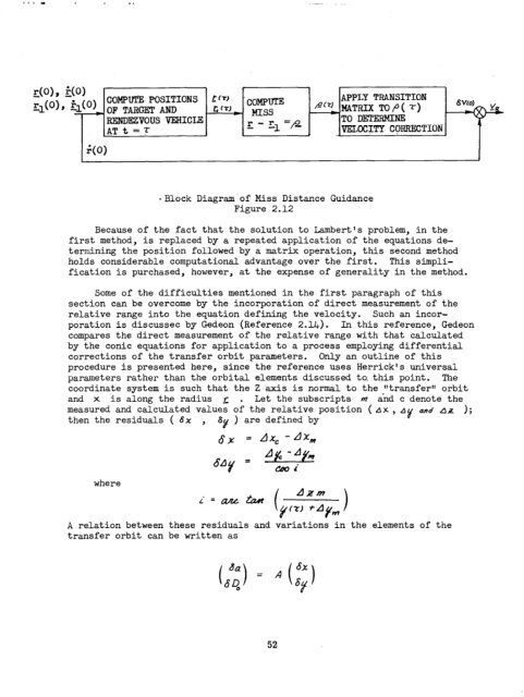
*Block Diagram of Miss Distance Guidance
Figure 2.12
APPLY TRANSITION
EtrCMATRIX TOP(r)
TO DEEIERMINE
VELOCITY C@RECTION
Because of the fact that the solution to Lambert's problem, in the
first method, is replaced by a repeated application of the equations de-
termining the position followed by a matrix operation, this second method
holds considerable computational advantage over the first. This simpli-
fication is purchased, however, at the expense of generality in the method.
Some of the difficulties mentioned in the first paragraph of this
section can be overcome by the incorporation of direct measurement of the
relative range into the equation defining the velocity. Such an incor-
poration is discussec by Gedeon (Reference 2.14). In this reference, Gedeon
compares the direct measurement of the relative range with that calculated
by the conic equations for application to a process employing differential
corrections of the transfer orbit parameters. Only an outline of this
procedure is presented here, since the reference uses Herrick's universal
parameters rather than the orbital elements discussed to this point. The
coordinate system is such that the 2 axis is normal to the "transfer" orbit
and x is along the radius r . Let the subscripts m and c denote the
measured and calculated values of the relative position ( AX, AY and 4~ );
then the residuals ( 6x , 8~ ) are defined by
where
6x = Ax, -Ax,
A relation between these residuals and variations in the elements of the
transfer orbit can be written as
52