guidance, flight mechanics and trajectory optimization

NASA CONTRA
REPORT
CTOR
GUIDANCE, FLIGHT MECHANICS
AND TRAJECTORY OPTIMIZATION
Volume XII - Relative Motion, Guidance Equations
for Terminal Rendezvous
by I>. F. Bender and A. L. BZackford
Prepared by
NORTH AMERICAN AVIATION, INC.
Downey, Calif.
for George C. Marshall Space Flight Center
; :* AFWL (WLfl-2)
j.@TLAND AFB, N MEX
NATIONAL AERONAUTICS AND SPACE ADMINISTRATION . WASHINGTON, D. C. . APRIL 1968

GUIDANCE, FLIGHT MECHANICS AND TRAJECTORY OPTIMIZATION
Volume XII - Relative Motion, Guidance Equations
for Terminal Rendezvous
By D. F. Bender and A. L. Blackford
Distribution of this report is provided in the interest of
information exchange. Responsibility for the contents
resides in the author or organization that prepared it.
Issued by Originator as Report No. SID 66-1678-4
Prepared under Contract No. NAS 8-11495 by
NORTH AMERICAN AVIATION, INC.
Downey , C alif.
for George C. Marshall Space Flight Center
NATIONAL AERONAUTICS AND SPACE ADMINISTRATION
For sale by the Clearinghouse for Federal Scientific and Technical Information
Springfield, Virginia 22151 - CFSTI price $3.00
TECH LIBRARY KAFB, NM
OOblllbb
P4vw3A Lfi- lull

- ..a --.

FOREWORD
This report was prepared under contract NAS 8-11495 and is one of a series
intended to illustrate analytical methods used in the fields of Guidance,
Flight Mechanics, and Trajectory Optimization. Derivations, mechanizations
and recommended procedures are given. Below is a complete list of the reports
in the series.
Volume I
Volume II
Volume III
Volume IV
Volume V
Volume VI
Volume VII
Volume VIII
Volume IX
Volume X
Volume XI
Volume XII
Volume XIII
Volume XIV
Volume XV
Volume XVI
Volume XVII
Coordinate Systems and Time Measure
Observation Theory and Sensors
The Two Body Problem
The Calculus of Variations and Modern
Applications
State Determination and/or Estimation
The N-Body Problem and Special Perturbation
Techniques
The Pontryagin Maximum Principle
Boost Guidance Equations
General Perturbations Theory
Dynamic Programming
Guidance Equations for Orbital Operations
Relative Motion, Guidance Equations for
Terminal Rendezvous
Numerical Optimization Methods
Entry Guidance Equations
Application of Optimization Techniques
Mission Constraints and Trajectory Interfaces
Guidance System Performance Analysis
The work was conducted under the direction of C. D. Baker, J. W. Winch,
and D. P. Chandler, Aero-Astro Dynamics Laboratory, George C. Marshall Space
Flight Center., The North American program was conducted under the direction
of H. A. McCarty and G. E. Townsend.

_- .-- ---
I

ABSTRACT
This Monograph is intended to present a discussion of the principles and
techniques of accomplishing a rendezvous between two spacecraft. In the con-
text here, rendezvous is considered as the interface between the midcourse
corrections of an orbital transfer maneuver which establishes the two space-
craft on nearly identical orbits and the docking maneuver which results in the
physical contact of the two spacecraft. First consideration in the discussion
is given to the development of the equations of relative motion of the two
vehicles. To facilitate the use in guidance scheme, these equations are
developed in various coordinate systems, with several choices for the inde-
pendent variables, and with several simplifying assumptions. Next, guidance
schemes are developed based on these equations of motion. As each guidance
scheme is presented, its existence is in some way justified and the relative
advantages and disadvantages as compared to the other schemes discussed. With
this discussion enough information is available so that the elements of a
rendezvous guidance scheme can be constructed for a particular set of condi-
tions in which a rendezvous maneuver is required.
NAA acknowledges the effort of the following persons in the preparation
of this Monograph.
Mr. H. A. McCarty, Program Manager
Mr. G. E. Townsend, Project Engineer
Mr. D. F. Bender, Author
Mr. A. L. Blackford, Author
Mrs. D. Chandler, MSFC Program Manager

110
2.1
2.1.1
2.1.2
2.1.3
2.1.3.1
2.1.3.2
2.1.4
2.1.4.1
2.1.4.2
2.1.4.2.1
2.1.4.2.2
2.1.5
2.1.6
2.2
2.2.1
2.2.1.1
2.2.1.2
2.2.2
2.2.3
2.2.4
2.2.4.1
2.2.4.2
2.2.4.3
2.2.4.4
2.2.4.5
2.2.4.6
2.3
2.4
2.4.1
2.4.2
2.4.3
2.4.3.1
2.4.3.2
3.0
TABLE OF CONTENTS
Page
STATEMENT OF THE PROBLEM. ...............
Equations of Motion. ...............
Coordinate Systems ................ 4
Field Free Case. ................. 6
Approximate Equations. ..............
Angular Forms of the Equations .......... ::
Distance Forms of the Equations. ......... 10
Solutions to the Equations of Motion ....... 13
The Out-of-Plane ................. 13
The In-Plane Motion. ............... 16
in-Plane Motion for Circular Target Orbit. .... i6
In-Plane Motion for Elliptical Target Orbits ... 21
Approximate Second Order Solutions ........ 22
The Effects of Perturbations on Rendezvous ....
Guidance Equations ................ ;:
Fixed Inertial Line of Sight (LOS) - Free Space. .
Manual Rendezvous Guidance ............ ;:
Separation of Guidance-Navigation Tasks. .....
Coriolis Balance ................. ;i
Improved Model - The Inclusion of a Gravity
Gradient .................... 37
Impulsive Rendezvous Techniques. ......... 39
Approximating Velocity Impulses. ......... 39
Two Impulse Rendezvous .............. 41
Extension to Non-Circular Orbits ......... 43
Multiple Impulse Rendezvous. ...........
Second Order Improvement ............. z
Direct Calculation using Two-Body Orbits ..... 48
Proportional Guidance. .............. 53
Optimization of the Rendezvous Maneuver. ..... 56
Optimal Stepwise Thrusting ............ 58
Optimum Power Limited Rendezvous ......... 71
Optimum Continuous Thrust Guidance for the
FinalManeuvers ................. ‘75
Free Space Model ................. 75
Linear Gravity Model ............... 80
RECOMMENDED PROCEDURES. . . . . . . . . . . . . . . . . 84
4.0 REFERENCES....................... 87
vii

a
b
aT
e
E
f
k
m
M
n
P
P
P,Q,h
-mm
r
5
R,B,Z
t
acceleration vector
LIST OF FREQUENTLY USED SYMBOLS
acceleration magnitude (of thrust)
sernimajor axis of target orbit
eccentricity
eccentric anomaly
force or control vector
fundamental matrix
transition matrix
angular momentum
Hamiltonian
switching function
mass
mean anomaly
mean motion
semilatus rectum
co-state variable
unit vectors centered at target vehicle describing an inertial
reference
radius vector from attracting body to rendezvous vehicle
radius vector from attracting body to target vehicle
components of cylindrical coordinate system centered at target
vehicle
time
ix

.
0
i
time difference between a reference time, to, and current time
unit vectors of rotating coordinate systems centered at the rendez-
vous vehicle
unit vectors of a rotating coordinate .system centered at the rendez-
vous vehicle
acceleration (control)
velocity
components along the u,v,w or u
--- -l,xl,wl unit vectors
.
components along the P,Q,W unit vectors
true anomaly
gravitational constant of attracting body
components of the relative position vector (e)
position vector between target and rendezvous vehicle
22
dt
3
dM
d
dB
d
dE
denotes a vector quantity
denotes a vector quantity
SUPERSCRIPTS
SUBSCRIPTS
denotes the ith component of a vector

1.0 STATEMENT OF THE PROBLEM
SATELLITE RENDEZVOUS
This monograph is directed to that portion of the rendezvous problem in
which the relative distance and velocity between an active spacecraft and a
passive target satellite must be reduced from moderate values (say 50 km and
5 km/set) to small values (say less than 5.0 meters and 1.5 meters/set).
&-board relative position and velocity sensing are assumed for the purpose of
allowing precise manual or automatic steering. These observed quantities are
to be utilized to drive the state of the system to zero in a reasonable time
with as little fuel as possible. Neither the gross orbital changes which have
been brought about previous to this closing (rendezvous) maneuver, nor the
final phase, known as docking, will be considered. The target satellite will
be assumed to be in a closed orbit; and since perturbative influences (such as
a non central gravity field) will be nearly the same on both vehicles with the
result that their effect will be very small, the orbit will be assumed to be a
two-body orbit, Since this monograph represents an attempt to survey the known
information regarding the rendezvous problem, it will be analytical in nature
and will not refer to any particular spacecraft or its capabilities.
The problem of station keeping is similar to that of rendezvous in that
it is assumed that a satellite is to be maintained in a specified orbit with a
specified phase within tolerances similar to those mentioned for rendezvous.
Thus, in a sense, the target is a point which moves along a desired path (this
path may not correspond to the motion in the actual gravitational field). On
the other hand, the chase vehicle moves along a path relative to this desired
path which is defined by the perturbative influences acting on the vehicle and
the differences in the positions and velocities. Accordingly, the position
coordinates of the chase vehicle may consequently deviate from those of the
target. After such a deviation has accumulated for a period of time the prob-
lem of returning the active craft to the nominal path in a substantially
shorter time is the rendezvous problem as presented. Of course, it is assumed
that the active craft possesses a mechanism by which the deviations from its
nominal trajectory are determined as they may be needed.
The discussions begin with the presentation of the field free case; i.e.,
the case in which the same gravity acts on both satellites. This problem is
of little physical importance; however, it serves to provide valuable insight
into a more rigorously formulated system. It might be surmised, at first
thought, that in this case no guidance technique would be necessary since an
astronaut could effect the rendezvous by line-of-sight thrusting. This would
approach would, however, cause the motion of the active craft to be one of
constant angular momentum about the target. That is, if an angular momentum
caused by an initial small velocity (v ) perpendicular to the line of sight
exists at the distance ro, then, if thg'distance is reduced to 10B3 r. and
1
-

only line-of-sight thrusting is used, the velocity perpendicular to the line of
sight will become 103v Thus, unless v is zero (initially), rendezvous
is not possible with &%-of-sight thrusti R g. For.the more accurate approximation
of linear terms in the equations of motion, the same situation pertains
except that some sets of initial conditions would reduce the effect and others
would magnify it. In either case, it is clear that a technique for managing
the relative velocity perpendicular to the line of sight and for reducing it to
zero as range and range-rate are reduced to zero is essential for rendezvous.
Further, though an astronaut could learn to make the necessary corrections by
trial and error, techniques for optimal and for automatic control are needed.
The rendezvous operation may be described as the overall solution to the
following set of interrelated problems:
a. The state determination problem.
b. The trajectory determination and prediction problem.
C. The trajectory control problem.
Each of these problems is discussed briefly here:
a. The state determination problem - Before making a course correction,
the current conditions (i.e., the orbit of the target vehicle and the
relative position and velocity of the active vehicle), must be deter-
mined. It is assumed in this monograph that this information, which
is taken to include error estimation, is available at the start of the
problem, as well as at later times as it may be needed.
b. The trajectory determination and prediction problem - the future sepa-
ration of the two vehicles must be predictable in some fashion in order
that changes of velocity can be determined which will cause the
separation to be reduced to zero at the same time the velocity differ-
ence is nulled. The degree of sophistication required in the equations
of motion will depend on the time to make the maneuver and the levels
of thrust that may be used. For times which are short compared to the
period of the motion and for thrust accelerations which are consider-
ably larger than the differences in the gravitational or other
perturbation accelerations between the two satellites, the motion of
the two vehicles approximates completely the field free space problem.
On the other hand, if the time to rendezvous is of the order of a
quarter of a revolution or longer, the equations must contain peri-
odic effects and secular effects produced by the dynamics of the two
bodies. However, since the object of the maneuver is to effect a
reduction of the relative motion to zero, it is to be expected that
approximate representations will be satisfactory as long as errors in
the rendezvous caused by poor representation at large values of the
relative coordinates can be corrected by subsequent thrusting as the
rendezvous is approached. In fact, this capability for error compen-
sation is required since noise and measurement errors in the data
sensed must be taken into consideration. Both the model errors and

the measurement errors could bdd to the fuel cost but under these
conditions would not hinder the eventually successful rendezvous.
The motion analysis in this monograph (Section 2.1) will not go
beyond that of linear terms in the relative coordinates, since these
terms are believed to be adequate for the ranges of relative motions
to be considered. A brief discussion of the possible effects of
perturbations due to air drag, earth oblateness, and solar-lunar
gravitation is included in the last portion of Section 2.1.
C. The trajectory control problem - Having determined the future course
and set up the capability of determining the velocity requirements to
effect rendezvous, a philosophy and a procedure to obtain it must be
generated, described, and shown to be successful. This development
of the guidance scheme is the heart of the problem. Thus, a series
of techniques which have been suggested for this purpose are described
in Section 2.2 (Guidance Equations). The rendezvous which is effected
with any given guidance scheme, however, may not be as close as
desired because of errors in the data and in the engine performance.
Further, rendezvous will not be optimal unless allowance is made for
the stochastic nature of the problem. Optimization techniques and
data filtering procedures will thus be important phases of the prob-
lem, and these will be described as found in the literature in
Sections 2.3 and 2.4, respectively.
For evaluation of the various schemes and for assistance in choosing
the state determination process, error analyses are required. The
work that is available in this area will be described in Section 2.4
Finally, in Section 3 suggestions for choosing the specific approaches
for a number of types of systems and the definition of interface
problems associated with mid-course orbital transfer or with the
final docking will be discussed.
3

2.0 STATE-OF-THE-ART
The significant analytical results concerning. the friendly rendezvous with
a passive target in orbit around a single attracting center are presented in
this section. The first portion (Section 2.1) deals with the equations of
motion and their solutions for coasting arcs and'for arbitrary powered arcs.
Some of the equations are used frequently as the coast.arc solutions (closed
forms) and are given (or referenced). The powered arc solution, on the other
hand, is reduced to a set of indefinite integrals containing the acceleration.
In Section 2.2 a series of guidance schemes is developed for the field
free and constant gravity field cases; a scheme is then developed for the
linear gravity gradient representations with their linear equations of motion.
In Section 2.3 the methods that have been used for optimization of the
rendezvous maneuver are discussed. Included in this development is a discus-
sion of optimal stepwise thrusting for time optimal, fuel optimal, and power
limited fuel optimal rendezvous and a brief discussion of optimal impulsive
rendezvous and its adaptation for finite thrust cases.
2.1 Equations of Motion
In order to formulate velocity requirements for rendezvous guidance it is
necessary to know how the relative motion of the target vehicle during rendez-
vous is influenced by the application of corrective thrust (to the spacecraft)
and by the passage of time for the case when no thrust is being applied. To
this end the equations of motion of the target with respect to the spacecraft
(as opposed to the absolute motion of the two vehicles in a central force
field),and the solutions to these equations are developed in this section. It
is noted that in a previous monograph of this series (Reference 1.1) the solu-
tions to the equations of relative motion are presented; however, since they
are to be examined in detail and since it is desirable to extend the material
in the reference to include sets of equations in terms of a variety of inde-
pendent variables, the equation will be re-developed here.
2.1.1 Coordinate Systems
The coordinate system for the relative motion is usually centered at the
target satellite and rotates with it. However, a significant simplification of
the circumferential component occurs if the unit vectors are determined by the
position of the active satellite. In this derivation, therefore, the reference
directions in the plane of motion of the target are chosen by the projection
of the position of the active vehicle onto the plane: the first axis (U)
being radial, the second axis (V) circumferential in the plane of the mztion,
and the third axis (W) binormal-to this motion. (At this point the oblateness
of the earth is neglected so that the target satellite moves in a truly peri-
odic orbit in a fixed plane.) The usual distance forms with the origin at the
target will be presented below in Section 2.1.3.2.
The target satellite is taken to be at the location
- r1
= rla where rl = ~(1 + e cos 81-l = aT(l - e cos E)=aTq 1.2
4

while the active (or chasing) satellite is taken to be at
r = rl(l + el) g + r1 5, x 1.3
where U lies in the orbit plane at the angle e2 ahead of U1, and where
!z r
51 9 53 are small angles while 52 is unlimited (Figure l.lT. Thus for
circular target orbits, the chase vehicle is allowed to be anywhere inside a
torus of small lateral dimensions centered on the orbit of the target. For
elliptical
so different
target
for
orbits
large
of high eccentricity, the values
t2 that tl could become large.
rl and r
Or to put it?EobtEer
way, if a torus of reasonably small cross section centered at the radius of
the semi-major axis of the target orbit does not include the whole elliptical
orbit in its interior, then 62 will have to be limited to moderately small
angles in order to keep [I small.
Figure 1.1 The Target Orbit Plane Vectors and Angles
5

Thus in cylindrical coordinates, the position of the target satellite is
(r' , 0, 0) and its motion satisfies the differential equation (the ' indica+es
d/dt)
while the active
satisfies
where a is the
ing rerZezvous.
p
the two satellites and 'is given by
/i’ = - pJp g,
--I
satellite is at i&(1 t [,I, B + e2, rl t31 and its motion
instantaneous acceleration produced by the engines in affect-
The differential equation for the relative position e= r - 3 is then
Agt 5 where Ag is the difference in gravitational accelerations of
Equation 1.6 may have a wider application than indicated here, for Ag may
represent the difference in all accelerations of the two satellites. Thus,
the reference trajectory could be a simple orbit satisfying any portion of the
total force equation. In fact, the idea of referring the motion of one satel-
lite to that of another nearby has been used in lunar theory since the time of
Euler in 1772; and it is doubtful if any of the sets of differential equations
given below could be considered to be original in this century.
The signs of the coriolis terms in equations found in the literature are
sometimes the opposites of those used in this monograph. The difference arises
from a difference in the choice of coordinate axes, here X radial, Y cir-
cumferential ahead; whereas many authors use X circumferential back, Y
radial.
2.1.2 Field-Free Case
For the field free case, the vector difference Ag is assumed to be
negligibly small and one obtains simply $ = 2 The solutions are immediately
available as
6
0
1.4
1.6
1.7

2.1.3 Approximate Equations
On the other hand, one may choose to obtain a set of linear
equations for the components of 4 which may be chosen in order
differential
to develop a
more accurate representation. This procedure will be adopted; but at the outset
it is desirable to point out that solutions to the homogenous part of
equations (i.e., for the case with no force, 01 that will be obtained are, in
fact, already essentially available. These are the state transition matrices
which have been discussed in the State Determination and/or Estimation
Monograph (Reference 1.1). Of course, independent '
variable changes and simple
coordinate changes will be necessary in order to obtain all the various forms
that may be used.
2.1.3.1 Angular Forms of the Equations
43
.
The expression for 2 = Y - 5 is developed in terms of r 1' 8, t,, 82,
and their derivatives by making use of
k=&, ~=64+$,_v, g =-bg , *ad -v =-(e'+ $ ),u. 1.9
The gravitational terms, expressed in components along g, x9 and W, me
The motion of the target satellite can be shown to satisfy
7
1.8
1.10
l.llb
l.llc

In this form the equations are valid to the second order in the e . It is seen
that the truncation of an infinite series (K) is required in only the radial
and the binormal component equations.
As already indicated, however, a linear theory is usually adequate for
rendezvous discussions; therefore, these equations reduce to the following set
of linear equations:
2-
where t7 -/a
-3
. 1.13
Here the independent variable is time; and as is customary, the dot indicates
differentiation with respect to time.
The first important point to note is that the out-of-plane motion is
decoupled from the in-plane motion, a feature that is characteristic of all
linear sets. These equations can be changed so that the independent variable
is the mean anomaly, M, since dM = n dt. This step is equivalent to making
the unit of time equal to the time required for a change ofoone radian in mean
anomaly. The resulting equations are (where the open dot is used to indicate
d/dM):
A major simplification occurs if the independent variable is changed to
the true anomaly, (@I, or to the argument of latitude (0 = 8 + 0,). The
transformation makes use of the conservation of angular momentum
8
1.12
1.14a
1.14b

Denoting d/d6 by the prime, ', there finally results:
For the case of coast arcs when al = a2 = a3 = 0, it is to be noted that the
out-of-plane motion is simple harmonic In terms of true anomaly and that the
first integral for the circumferential equation can be written down at once.
Another form of the linear equations of motion which will be considered
makes use of the eccentric anomaly, E, as the independent variable. To
accomplish this transformation, the substitution
is made where q = 1 - e eoe E = 'l/aT and u = -6-z
where
with the asterisk, R ) there results:
equals the acceleration of gravity at the distance of the semi-major axis. For
coast arcs the third equation is easily integrable as will be shown below, and
the second equations possess an immediate integral as for Figure 1.16.
9
1.16a
1.16b
1.16~
1.17
1.18a
1.18b
1.18~

For all the equations given to this point, the reference orbit can be
elliptical. If the path is circular, a further simplification occurs for each
form presented. The set with time as the independent variable (Eq. 1.12)
becomes (rl = r. = constant):
The remaining sets (Eqs. 1.14, 1.16, and 1.18) reduce to a single set because
of the equality of the three anomalistic variables (M = 8 = E) for circular
orbits. This set is
It is to be noticed that for linear systems and a circular reference orbit
the set of equations has constant coefficients and is, therefore, easily
integrated for the case of coast arcs (g = .- a = 2).
As already mentioned for the. sets of equations in terms of true anomaly or
eccentric anomaly, the second of the three equations possesses an immediate
first integral for the no-thrust situation. This integral is a representation
of the constant difference in the angular momentum per unit mass for the two
vehicles. Thus, for the no-thrust case, there must exist three more independent
integrals consisting of simple combinations of 51, t2, 6'1, rt2 represent-
ing constant differences in other elliptical orbit elements (e.g., semi-major
axes, arguments of perigee, times of perigee passage). This concept, in fact,
yields a method for obtaining the integrals to the sets.
2.1.3.2 Distance Forms of the Equations
In the first place, let
10
1.20b
1.2oc
1.21a
1.2lb
1.21c
1.22

and assume an elliptical reference orbit. Note that the reference system is
centered at the target. Now, using the derivative of UJ and xl as in
Section 2.1.3.1 the equations are found to be:
Note that moving the origin to the target vehicle has the effect of causing a
K term to occur in all three equations. The second-order form of these equations
as used by Anthony and Sasaki (Reference 1.2) is obtained by introducing
changes of scale for both distance and time. In.this reference, the semi-major
axis, aT' of the elliptical
thus, x = aTX19 y = apl$
to mean anomaly, M, and
reference is used as a normalizing variable;
z = aTzlt and = aTq. The time is then changed
d/dM is represente 'a with the open dot, O, as
before. Including the second-order terms on the right, the equations become:
For circular orbits the equations simplify to equations of exactly the
same form as Equations 1.20 thus 'indicating the equivalence of the two origins
(either active or target) for rendezvous. Thus, one finds
2-3n”x -2nj =a,
Y
+Zfl;r: =a Y
it + n2t =a *
For the final two forms of the equations, consider that 2 is expressed in a
set centered at the target in an elliptical orbit and oriented in a fixed set
11
1.25

of inertial directions which are taken to be those of perigee (P), Q = WxP
and W (binormal). First choose a rectangular set (Figure 1.2)-wheFe --
The result is:
Here, of course, the terms involving p are the first linear terms in the
series expansion of Ag.
Finally, using a cylindrical set of coordinates (R, 'I', 2) where
kZ= R&s the equations are seen to be
From sets 1.26 and 1.27 the usual expression for circular reference orbits is
obtained by substituting nz '//fl,3
Figure 1.2 Target Centered Coordinate Systems
12
1.26
1.27

2.1.4 Solutions to the Equations of Motion
As has been mentioned in the discussion of the state transition matrices
of the State Determination Monograph (Reference 1.11, this matrix represents
the solutions to the homogeneous parts of various sets of the equations. However,
rather than refer to them directly, solutions will be developed making
use of matrix methods in this section; especially since it is desired to
include the effects of the thrusting acceleration, a3. The sets of equations
will be sp&&mto - \- the out-of-plane motion and the in-plane motion. Further-
more, the techniques of the matrix method will be illustrated in the solution
for the out-of-plane motion; since this motion is seen to be simple harmonic
motion with a forcing function (except when the reference orbit is elliptical
and the independent variable is eccentric anomaly). Matrix methods and results
are given by Leach (Reference 1.31, Tschauner and Hempel (Reference 1.4) for
circular reference orbits and by Tschauner and Hampel (Reference 1.5) and
Tschauner (Reference 1.6) for elliptic reference orbits.
2.1.4.1 The Out-of-Plane Motion
The out-of-plane motion can be represented by the differential equation
for all cases except the set Equation 1.18, which will be considered later.
The matrix methods require that the equations be expressed as linear first-
order equations. This is accomplished by de.IYni.ng the two vectors 5 as
Thus, Equation 1.28 becomes
where
t=(;j = (2)
and 8 =
To proceed, the fundamental matrix (F) for A must be found; that is, a set
of independent solutions to
1.29
1.30

which form the columns of F must be found. This process is difficult in
general; thus, sometimes it is preferable to make a transformation of variables
to simplify the matrix A before attempting to find the fundamental matrix F.
For the present equations, however, the solutions are known; and the fundamental
matrix can be written in terms of real functions as
The inverse matrix is
Now, since
d(f"f)
09
F--k9 = l iant 41 cmnt
cmnt -h&d )
=o , it is easy to show that
f (f-9 = +-‘A
for all problems of this kind. In order to obtain the solution, it is conven-
ient to obtain a set of constants for equations with no forcing (a, =O). This
is accomplished by the substitution
which is seen to satisfy the differential equation
1.32
1.33
1.34
3 = F%)5 1.35
i =‘F-‘(t) B o3 U)//l, 1.36
This equation is integrated to give Z - Z, and is then multiplied by F(t)
on the left to obtain the original variable, 5 . The result is
The state transition matrix for these two variables is F(t)F -l (t 1. When the
coefficients in the matrix A are constant, it is possible to wriee
F(t) F -‘Cl, ) = G (t - 4,)
14

For this case (t - to = T)
This solution, valid for circular reference orbits, is also applicable to
elliptic reference orbits by changing nt to 8 which is then true anomaly.
The solution to the out-of-plane problem for the case of elliptical target
orbits and eccentric anomaly is given by Tschauner (Reference 1.5). Let
Thus, the set becomes
where
The fundamental matrix is now
and
In this case, the substitution
and
z =F-'La&
gives the equation (q = r/a = 1 -e Cos E)
15
1.39
1.40
1.41
1.42
1.43

Thus, the solution is written
The transition matrix then becomes
F(,L)F-‘(El = k Lz% 3
where a and b are defined by the equations below:
a = wo (L -6) -e(cooE+mEo) +e2(/-dirCE&Eo)
2.1.4.2 The In-Plane Motion
2.1.4.2.1 In-Plane Motion for Circular Target Orbit
For the case of the in-plane motion and the circular reference orbit, the
first two equations of Equations 1.21 are used. To express these as a set of
linear equations, let
The set becomes
16
1.44
1.45
1.46
1.47a
1.47b
1.48
1.49

where
A= B=
The characteristic equation for A is A4 + A2 = 0 from which it is seen
that the four independent functions out of which solutions are formed are 1,
0, sin 6, and cos 8. The fundamental matrix may be'taken to be:
(
F(0)=
0 1 -30 -3 2 0 cos Sin 2 -2 cos Sin 6 8 0 8 cos -2 Sin cos Sin 8 6 8
1.50
The determinant of F is equal to unity,and the inverse is
1 -2 38
0 0 1
-3 case Sin6 0 -Sin@ case -2 cos Sin 0 8 >
Thus, making the substitution
z = F-‘(e)[
allows the differential equation for Z to be written as
or
Z' =
( -Sin
z’ = F-‘(e) B(;)
2 cos 0 8 -2 1 38 cos Sin e 8 )
The state transition matrix for the variables y is thus
Fce,F-?q = G(8-8,)
17
1.51
1.52
1.53
1.54

This matrix is simply written as G(8) (i.e., this notation is used to avoid
writing)
4-3 cos 8 0 Sin 6 2(1 - cos e)
6(Sin 0 - '3) 1 ~(COS 8 -1) 4 Sin e - 3
G(8) = 3 Sin 0 0 cos 0 2 Sin 8
6(Cos 8 - 1) 0 -2 Sin 6 4 cos 0 - 3
This matrix, when combined with that of Equation 1-38 and both expressed in
terms of 8 = nT (and n added as needed to give dimensions correctly), are seen
to be exactly that of page 145 of SID 65-1200-5 (Reference 1.1).
In the case of the representation of state transition matrix for locally
level inertial systems (Table 2.4.2, page 147 of Reference l.l), the coordinate
transformation required is only that between inertial and rotating systems at
the moment they are aligned. Reverting to 6 = nT, the rotation rate is one of
the angular velocity, n, about the z or third axis and the transforma-
tion matrix, T, for 6 =TX is
with
T = [
‘&
---d- I ' 0
1
0 -n!
n o!I
The state transition matrix for inertial locally level (at both times) may thus
be obtained from G(nT) and it is Q!
'1
= T'lG(nT)T =
:
2-Cos nT sin nT l/n Sin nT 2/n(l-Cos nT)
2 Sin nT-3nT 2 Cos nT-1 2/n(Cos nT-1) l/n(4 Sin
n(3nT Sin nT) n(l-Cos nT) 2-Cos nT 3nT-2 Sin nT 1.58
n(Cos MT-l) -n(Sin nT) -Sin nT 2 Cos nT - 1
The development of the system by Tschauner and Hampel (Reference 1.4)
involves a substitution to simplify the matrix of coefficients. In addition,
the out-of-plane motion will be included and the set of six equations solved
with matrix notation for later reference. It is simplest to add the out-of-
plane coordinates to the set of four in-plane variables of Equation 1.48 as
18
1.55
1.56
1.57

The set of differential equations is now written as
W’ = Awtf
where the transformation from the position and velocity differences

The fundamental matrix for A can be written at once as
10 0 0 .O 0
8 1 0 0 0 0
0 0 cos 8 Sin 8 0 0
F(0) = 1 0 0 -Sin 8 cos 0 0 0
for which the inverse is
0 0 0 0 cos 8 Sin 8
0 0 0 0 -Sin 8 cos 0
F-‘(e) = F(4)
The solutions to the equations can now be written in the form
In this case, the matrix G(0 - Go) = F(B) FD1(Qo) is easily seen to be
-
1.60
1.61
GM-8,) = F&J-q) 1.62
Note that F(Oj = F-l(e) = I. In fact, since no loss of generality occurs
by choosing 0, = 0, this value will be assumed for the remainder of this
section. The six integrals in the solution for w (0) (called "Z"> will be:
2, =
s
0
8
u2 d-r
e
I- =
J
(73 f32y)d7-
0
1.63

Finally, the solutions are expressed as
To repeat,the boundary conditions at 8 = 0 are w = w. and are seen t: be
satisfied. The final boundary or rendezvous conditions at 0 = Bf are (? =
WT = (0, 0, 0, 0, 0, 0).
2.1.4.2.2 In-Plane Motion for Elliptical Target Orbits
A technique for obtaining the solutions to the in-plane motion has been
mentioned (Section 2.1.3) and references made to two papers by J. Tschauner
(References 1.5 and 1.6). It is suggested that these papers be reviewed as
required; the ability to obtain these solutions should allow a completely
satisfactory representation of the problem of rendezvous with targets in
elliptic orbits.
21

2.1.5 Approximate Second Order Solutions
A solution to the equations of relative motion which includes both
linear and quadratic terms in the gravity expansion and which is applicable
to target orbits of small eccentricity is developed by Anthony and Sasaki in
Refarencz 1.2. This work is essentially a combination'of the work of London
(Reference 1.7) who examined the effect of including the quadratic term for
circular target orbits, and that of deVries (Reference 1.8) who considered
target orbits of small eccentricity, but included only linear terms in the
gravity model.
The equations of motion are given in terms of a rotating coordinate
system centered at the target as in Figure 1.2. The equations
before any approximations are made, were developed previously
of motion,
in time of
non-dimensional variables as Equation (1.22). For convenience
reproduced below-along with the definition of the non-dimension~
this set is
variables.
where
and where the open dot superscript (e.g., 2 ) refers -to differentiation with
respect to M. Expanding the nonlinear terms of the differential equations in
powers of the coordinates and retaining linear and quadratic terms results in
the set.
(1.66)
NOW, for orbits of small eccentricity, the variation of 8 and p with time
(and ultimately with PI) can be written as a series expansion in the
eccentricity, e,.g.
8 = /fZcz wdt-t*)
22
(1.67)

where the subscript 70 refers to the condition at the time of periapsis
passage.
If the nonlinear terms are omitted and the target orbit is circular,
Equation (1.66) is identical to Equation (1.49) and a solution for x, y, a
can be found in terms of the initial conditions x,, yO, zO, 4, fO, &, by
.the use of the transition matrix Equation (1.58). If this solution is de-
noted by the subscript 1'~" then
The solution to the nonlinear equation will be defined in terms of this
solution and small corrections; that is, the solutions to the set (1.66)
have the form
If this solution set is substituted in (1.66), a set of differential
equations for the variables 6~ , 6% , and 62 is produced. This set is
then simplified by neglecting the s;naller terms such as x,6x , =6x ,
ec , eZv, etc. The resulting differential equations are
8.2 +8-i? = 3~52, -3ezc cfm(r-7,)
This set of equations is linear in terms of the known. forcing functions;
therefore, the solution is straightforward. For convenience the solution is
given in two parts indicated by
where the superscript 0 denotes the solution when the target orbit is
circular, and the superscript e denotes the effect of small eccentricity on
the solution. These solutions are given by
Sxp=Aof + /f&n z +/~+KI r tAjP& 2 r +/4~cooZ r + A5%.
23

where the superscript p can be either o or e.
are then given by
24
The constants A: , B' Cj
i '

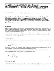
A comparison of the linear and quadratic solutions is given in Figure 1.3,
1.4, and 1.5, (from Reference 1.2) for a target orbit with apogee and perigee
altitude of 400 miles and 200 miles. The figures were generated by assuming
the relative position was zero at time zero, but that a non-zero relative
velocity existed as indicated on each figure.
Figure 1.3
Comparison of Linear, Quadratic, & lkact (Numerical)
Theory for 100 FPS Velocity Increment
27

w”
2
E
IOOJ-
-100
- 200
AV = 400 FPS
I I Pip
-400 \ x
-wo.p)d
-600
I
I 1
0 lk 2x 3Yr
I
-200
-400
-600
ifi
2 -800
I
2
- IO00
Figure 1.4
Comparison for Velocity Increment of 400 FB
-1200
-1400
0
I 1
AV = 400 FPS
As expected, the linear solutions are accurate for a short time until the
distance involved becomes large. This divergence occurred in approximately
l/2 revolution for the trial cases. Thereafter, the linear results differ
substantially from the actual (numerical) solution partically in the vertical
component. The quadratic analysis yields accurate results for approximately
two revolutions of the target.
28

ii
2
I
2
4!m
4000
3500
3000
250C I-
rood I--
)-
I-
I-
‘5
0 CUAORATIC THEORY
P LlhEAR THEORY
-
-
AV
AV -827.52 FPS
Figure 1.5
Extreme Case Comparison
Figures 1.5 illustrate a rather extreme case of velocity difference in
which even the quadratic theory breaks down rapidly. However, even if this
case for relative distance is less than 2500 miles, the predictions are quite
accurate.
2.1.6 The Effects of Perturbations on Rendezvous
Satellite orbits are perturbed from pure conic sections by forces due to
the earth's atmosphere, the non-sphericity of the earth, the attraction of the
moon or sun, and the radiation pressure of solar radiation. As was indicated
earlier, the term A g really represents the difference between the accele-
rations of the two objects due to all forces. The earth's atmosphere could
29
3n

cause a significant effect for rendezvous maneuver sufficiently low, but the
assumption iz this study is that the maneuver is as a suf.ficiently high
altitude.( >150 Km) that air drag is negligible. The largest of the
remaining forces in th's region near the earth is that due to the oblateness
of the earth. The magnitude of this force is about 10-3 times that of the
inverse square force and while its gradient coefficient is twice that of the
ma-in term, it is clear that the magnitude of the contribution to Ag is not
more than l/500 that of the main term which is itself expressed only approxi-
mately. Consequently,.all perturbative differences can be safely neglected
in studying rendezvous in orbits near single attracting centers that are no
more oblate than the earth. Rendezvous in earth-moon space is thus considered
in the monograph only if near enough to ona of the attract?ng centers, that
the perturbative force due to the other is substantially smaller than the
main gravity turn.
2.2 GTJIDAVCE F,QUATIONS
In this section the methods that have been proposed for mechanizing the
rendezvous are presented. 19 several cases , guidance schemes are chosen without
regard to the degree of optimization;-however, when the a preach is taken,
tlie considerations will be detailed L see Section (2.L) 4 -,
2.2.1 Fixed Inertial Line of SFuht &-CC] - Free Space
~ --__ - _____C_.__._
-_- ..a--.. . ..--.---1_
It has been shown in a previcus section that the Vatural.'t maneuver of
thrusting f-n the direction of the T,c)S w-X.1 not, in general, produce rendezvous.
However , for the special case with the relative velocity vector aligned
parallel to the LOS, then thrust thrusting along the LOS is the optimum
method of achieving rendezvous (in free space). This fact is demonstrated in
Section 2.4 where optimization is discussed. This solution suggests that a
mar.euver which first orients the relative velocity vector along the LOS
could be advantageous. Aligning the velocity vector in this way is equi-
valent to nu13ing the angular rate of the LOS in inertial space'and can be
acccmplished by appldg thrust normal to t!?e YE. The overall maneuver,
+.'lus, retains a degree of naturalness in that an astronaut performing a
man-la: rendezvous can easily determine the directions in whFch the thrust
i 9 t 0 be applied.
The discussion Fresented here is limited to its application as a manual
hack up guidance technique for Gemini as presented in papers by Chamberline
and Rose, and Burton and Ha.yes (References 2.2 and 2.3), and to an extension
cf the technique by Steffan (Reference 2.4) which separates the guidance and
navigation tasks. Because of the approximation that there is no relative
acceleration due to gravity, the range of initial ccndjtjons for which this
t.ec~njql~e has acceytab1.p accuracy is limited. A larger set of initial
conditions can he handled if a number of fVmidcourse 1' correctinns are made.
nowever, fr-m a-? eff; ciency st.andpoin+.,
undesirab!e. The nri.ncina! I advantaee
a natural basis for manual gui.dance.
these midcourse corrections are
of th5.s method lies in its use as
30

2.2.1.1 Manual Rendezvous Guidance
The technique of fixing the direction of the line of sight in inertial
space effectively uncouples the linear and angular motion and reduces the
problem to one dimension. This feature is a particularly useful in the case
where a pilot is manually performing the rendezvous. Such a system is con-
sidered as a back-up for the Gemini missions (Reference 2.3); for the Gemini
scheme, the pilot visually observes the relative motion between the spacecraft
and the target vehicle with respect to a star background. Range and range-
rate information are provided by radar or optical means. When the two ve-
hicles are within a preselected distance, the pilot initiates a thrust
maneuver normal to the line of sight until he observes that the relative
(angular) motion has been eliminated. This process is continued throughout
the rendezvous whenever relative motion is again noticed. The range and
rate range are monitored so that the time to begin the braking maneuver can
be determined.
2.2.1.2 Separation of Guidance-Navigation Tasks
In the previous section, the astronaut performing the rendezvous maneuver
was required to navigate (i.e., determine when the relative motion has ceased)
during periods of thrust application. A technique developed by Steffan
(Reference 2.4) determines the time duration of the thrusting from data taken
before thrust initiation. The angular rate of the LOS is allowed to oscillate
between limits with the period of oscillation determined by thrusting in the
LOS direction. This technique requires the application of several velocity
increments normal to the LOS, the times of these applications are related to
the period of the limit cycle and are controlled by controlling the range
rate. The desired period of the limit cycle is then chosen so that the time
between corrections is sufficient to allow for data taking and processing.
This time will vary depending on how the data is being taken and processed,
e.g., a range radar feeding information directly to a computer vs. optical
measurements and hand calculations by an astronaut.
By the use of the rocket motor normal to the LOS, the rendezvous ve-
hicle is established on a collision course with the target vehicle such that
the direction of the LOS is stabilized, to within some limits, in inertial
space. The approximate behavior of this limit cycle can be determined
analyzing the expressions for the angular rate of the LOS as a function of
time for (1) termination of normal thrust and (2) time for the initiation of the
normal thrust. First the case of no thrust is considered.
A polar coordinate system will be used to describe the motion. In this
system, the range (p) is defined as the distance from the rendezvous vehicle
to the target vehicle; a' is measured from an inertial reference direction;
and the origin of the coordinate system is at the target vehicle.
31

Figure 2.1
Polar Coordinate System
(Since the out-of-plane motion is uncoupled, only motion in two dimensions
is considered.) Now, since for the case under consideration, there is no
relative acceleration between the two vehicles due to the gravity gradient;
thus the angular momentum of the system will remain constant (for period of
no thrust). i.e.,
The subscript, o, refers to some initial time. Therefore, if the normal
control has been operating, the velocity vector will lie along the line of
sight (to the first order) and the range as a function of time will be
With the use of this expression for range, the angular momentum equation can
be written as
2
sw (,+$t)?
Equation (2.3) is the desired relation for the angular rate ( b ) of the
LOS for periods of free motion.
32
0
(2.1)
(2.3)

p
The kinetic energy of the system is
Thus, Lagranges equations of motion for periods of normal thrusting are seen
to be
where a,, is the acceleration due to the normal thrust. Now substituting
relation for p as a function of time from Equation (2.2) in the second
equation above gives
or
This equation can be considered a first order differential equation in the
variable 4 , i.e.,
But this equation has as a general solution
Equation (2.4) is the solution for the angular rate of the LOS (e ) during
periods of normal thrusting. This equation, however, is not the one employed
to determine the length of time that the normal thrust is to be applied, but
rather the simpler equation which assumes ,d '= 0 is used. The time of normal
thrusting is calculated as
l
That is, if T0 is the threshold
to zero the length of time that
A? ?3
(2.5)
tn = -
an
.
value of t and it is desired to drive 8
normal thrusting should be applied is calculated
from (2.5). If the motor used for normal control is actually operated
for this time, 8 will not be driven to zero. Rather, the value that it
33
(2.4)

.
will attain, z , can be calculated by substituting the value of t, from
Equation (2.5) into Equation (2.4). This substitution gives
Thus, assuming l&j L4 Ia,1 (this approximation becomes better as
r-0 as will be seen when motion along the LOS is discussed) the ex-
pression becomes
The overall behavior of 6 can thus be determined from this equation and
from the one given earlier for a no-thrust condition L Equation (2.3)].
This overall behavior will be a limit cycle between the values f0 and x
as characterized in Figure (2.4). The time between applications of normal
thrust ( tc) and fl can be
calculated from Equations (2.3)
and (2.6). Letting z= -$
(the time until rendezvous
occurs assuming no radial
thrust is applied) quation
(2.3) results in
a'Limit Cycle
Figure 2.2
Finally, substituting for Z$ from Equation (2.6) gives
A certain minimum time will be necessary to take and process the data
to determine the current position and velocity. Therefore, it will be
necessary to require that the time between corrections, t,, be longer,than
the minimum data taking time. Since p is to be driven to zero and F, is
small, it can be seen from Equation,(2.7) that a minimum t, will be maintained
ifaminimum 1 is maintained. In turn, a constant7 ( or more practically
a constant range of values for T ) is obtained by a proper choice of
thrusting periods for the LOS thruster. A discussion of motion along the LOS
is now called for so that the behavior of 2 during periods of LOS thrusting
34
(2.6)
(2.7)

‘i
can be determined.
If the angular-rate control system is operating, the approximate
range-rate and range equations for periods of LOS thrusting are
where a1 is the acceleration along the line of sight. The corresponding
expression for r is thus
and
If the desired limits of z are rrn," L t L -zmaX
(2.8)
dT
and if the slope zt
is positive at t = 0, then the LOS thrusting is initiated whenever Z-L r,,,
and terminated whenever r = rm,, . If the slope of $$ is negative at t=O,
then I will continue to decrease up to the point at which $z changes sign.
(Figure 2.3) In this case, the minimum value to which + will be driven
must be predicted so that
thrusting can begin
sufficiently early to
r
prevent 2- = T,,, .
The point at which
reaches its minimum
value is determined
by solving Equation (2.8)
with cft C-= = 0 . The result
is
r -- ----___
mm
k
A
Motion of T
Figure 2.3
.?
IN”
=; [-/j -.!Y]
and the corresponding value of 7;r,,, obtained by substituting this time is
the equation for 7 is:
35

This equation may now be solved forp,
lower limit)
and replacing rm by 2-,,, (the desired
Thus, for the case when the initial slope '$ is negative the motor is fired
whenever this equation is satisfied and firing is terminated whenever
T- t ~mor . If this scheme is used to control the velocity along
the line of sight, the time until rendezvous will remain between the limits
f -,- and Ge and the range will be forced to decrease approximately ex-
ponentially with time. As the range becomes sufficiently small, the range
rate control loop is opened and a docking maneuver initiated.
2.2.2 Coriolis Balance
The two previous sections considered guidance schemes based on nulling
the angular rate of the line of sight. In this section, a technique where
the line of sight is allowed to rotate at a constant rate is considered. It
will be seen that this restriction is equivalent to requiring that the force
normal to the line of sight be equal to the coriolis acceleration. Hence,
the descriptive title "Coriolis Balance". (Reference 2.5).
Using a polar coordinate system centered at the target vehicle and
assuming no relative gravitational acceleration, the equations of motion
are (as in Section 2.1)
Now, if the LOS acceleration, aR, equal to zero and the normal acceleration
is equal to the coriolis acceleration ( a,, = 2,6 2 ) these equations
become
p-p&'2=o
But, the second equation shows that the angular rate is constant and that the
range equation can be written as
(2.9)
/i--s2p =o $ $=a”= CONSTANT (2.10)
Equation (2.10) nOh’ shows that the coriolis balance technique also uncouples
the angular motion from the range motion. The problem is now to show that a
collision will result if this acceleration is applied. Consider the solution
to Equation (2.10) at the boundary p = 0.
36

This equation ;zill have a solution for positive time, if 4'0 and IAd\ pp6 .
If these conditions are not met, or if the time to rendezvous is unsuitable,
a velocity impulse along the line of sight can be added to remedy the
situation.
The solution to the Equations (2.9) for an acceleration is applied along
the line of sight (uR) is now
If the conditions for rendezvous (i.e., P =o, p = 0) are inserted in
these equations, it can be seen that a solution can be obtained for a,
equal to a constant. Thus, the rocket motor A~rn+sh~nrr thrust along the line
of sight need not be throttleable. However, the normal thrust motor must
furnish thrust according to
and is therefore required to be throttleable.
The author or Reference (2.5) compares this scheme to a scheme which
nulls the angular rate similar to that described in the last section. The
comparison indicated that the coriolis balance technique requires a lower
thrust level for both the range and normal rocket motors; however, the total
impulse and flight time are greater.
2.2.3 Improved Model - The Inclusion of a Gravity Gradient
An improvement in the description of the gravity model can be made which
will increase the range of initial conditions over which the preceding methods
are valid, yet still retain the simple expressions for determining the
duration of thrusting. The improved gravity model consists of approximating
the difference in the gravitational acceleration of the two vehicles ( A$ )
by
37

If the matrix 121
model discussed'&
is taken as a function of time, then the linear gravity
Section 2.1.3 can be applied. However, the matrix can be
approximated by a constant for short time periods and a less than precise
gravity model suitable for improving the free space model is obtained. The
value of the constant matrix can be obtained as the average value of (%/ae)
during the thrusting period, i.e., if K denotes the constant value which
approximatess($/a,)then
h
fi)
A?= Or
&
ar
dt
f
Using this approximation, the equations of motion are
0
A solution to this equation is easily obtained if it is rewritten as set of
two first-order equations
then
or
where
The solution for Y is
y=e Af Y(O) +fkBo d+
In the previous sections, only the integral term on the right hand side of the
above equation was obtained. Thus, the only modification to the equations
developed in those sections is the addition of the expression involving the
initial conditions. Mechanization is, thus, similar.
0
38

2.2.4 Impulsive Rendezvons Techniques
-.. - ---I--.-----.
Tn thi.s section, the development of guidance equations in a linear
gravity field will be restricted to determining an impulsive velocity
correction such that a rendezvous till take place at some time in the future.
The techniques of this secti.on can be thought of as defining a reference
trajectory along which the rendezvous vehicle is to travel. Once this
reference trajectory has been established, the actual steering equatinns
(i.e., orientation of the thrust vector as a function of time) can be
determined by the methods discussed in a previous monnqraph of this series
on boost-guidance equations (Reference 2.16). The section below gives a
discussion of two simp3.e techniques for utilizing cal cu!.ated velocity impulses.
Impulsive velocity changes have been considered in detail in the
monograph on mi.dcourse guidance (Reference 2.15) and this reference is
recommended for a more com@ete formulation including the effects of errors
in data and optimization of mu!.ti.ple i.rnpulse schemes.
2.2.4.1 Approximating Velocity Impulses
The use of a model having a linear variation in gravity generates the
necessity of neglecting the effects of finite bnrning time in order that
closed form solutions be obtainable. Al though, th,e use of imp111 sT.ve
ve3 ocity changes is essential to the simoV fication of the equ,ati ons, their
physical realjzation can be only anproximate. If a true impulse could he
achieved, then the guidance mechanization won!d simply be to orient the
thrustor along the direction of the required vel.ocity chanece and apply an
impulse equal to the magnitude of the required chance. Since th.e rocket
motor must bllrn for a finite time (the length of t?me depends upon the
thrust capability in relation to the magnitude of the velocity increment)
the orientation of the required veloci.tg increment will., generally, nnt
be the same at the initiation and termination of the thrusting period.
Thus, if the rocket
v
!ENDEZVOUS
VEHICLE ORBIT
Figure 2.4
Di.rection of Velo&tp Correction
TRAJECTORY
Rocket motors were oriented along the required AV vector and maintained in
that orientation throughout the thrusting period, the resulti.ng velocity
increment wnnld have the correct magnitude, but it would be directly incorrectly.
39

One method which can be employed (and has been employed in the Gemini
missions (Reference 2.3))t o compensate for the finite thrusting time is to
center the thrusting period about the time at which the velocity impulse is
to be applied. For example, if it is calculated, that the velocity change
to be applied at t = to to achieve rendezvous is AV, and the acceleration
produced by the rocket motor is T/M then the length of time the motor is
required to burn is
The thrust period'is then centered about time to by initiating the thrust at
&=

This updating can be accomplished, however, at a much slower rate than is
necessary for steering and cut-off calculations. In the reference, Gunckel
proposes to update one element of the matrix each computation cycle; thus,
updating the complete matrix in nine cycles. Since the quantities under the
integral sign are taken to be constant during the time period, the above
equation can be written as
2.2.4.2 Two Impulse Rendezvous
The first linear impulsive guidance scheme to be considered was pre-
pared by Clohessy and Wiltshire (Reference 2.1) and is the basis of the
Gemini automatic rendezvous guidance (Reference 2.2 and 2.3). Two major
velocity impulses are used through several smaller mid-course corrections
calculated from the same equations and based on intermediate measurements of
the state attained by the first change in velocity may also be required.
The first velocity impulse is applied at the beginning of the rendezvous
maneuver and establishes the target and rendezvous vehicle on a collision
course. The second impulse is required to null the range rate at the time
of closure. Consider a target
vehicle in a circular orbit and
a coordinate system fixed to the
target such that the Y axis is
always along the radius from
the center of attraction, the
X axis is circumferential inthe
direction of the motion of
the target, and the Z axis
completes the right handed
XYZ set. If the rendezvous
vehicle is in an orbit which
closely approximates that of
the target vehicle, then the
transition matrix of Equation
(1.58) can be used to describe VEHICU
the relative motion. In this Linear Rendezvous Coordinate System
I scheme, the only concern is the Figure 2.5
reduction of the range to zero;
thus, the only part of the matrix which is needed is rewritten below.
41

If a collision is to occur at time r then the components on the left of
this equation must be zero. If this substitution is made and the matrix
multiplication indicated on the right performedi the three resulting
equations are
assuming that the position at t = 0 is fixed, the velocity necessary to
achieve a collision at time 'f can be determined by solving the above sets
of equations for X0, Y,, and Z,.
2d = nZo coYnr -4
Thus, if the rendezvous vehicle is at a position (X0, Y,, Zo) with velocity
lVXo' vY '
V
z,
) and the desired time to rendezvous
velocity'increment necessary is given by.
is -r then the impulsive
"$=4-v,
AVy=i -‘I,
Av,=r, =s 0
The velocity which must be nulled by the braking impulse can now be determined
by again app$ying the transition matrix to the initial conditions
x 0’ Yo' Zo' X0' yo, Zo'
=3n&nr&
%-
+won7-ia +ZAnZk;~
A
= 6n(mnr-i).Zd - Zdinnr20 f fC(CdOnT-3)fi
kr = -nknrr, +c&-onT2*
Note that this method requires knowledge of the time at which rendezvous
is to occur. However, there are several factors which will indicate a
suitable choice for 5 . For example, in the Gemini rendezvous, it was
found that the velocity requirements for a rendezvous maneuver which caused
interceptions in three-fourths of an orbit were less than for other fractions,
therefore, r is chosen to cause such an interception (Reference 2.2).
Another criteria would be the adjustment of the closing rate to be compatible
42

with the rocket motor which is to supply the braking thrust. Data taking
and processing requirements could also place a particular requirement on .
For a generalization to finite thrusts, see below Section 2.3.1 and the work
of Tschauner and Hempel (Reference 1.k).
2.2.4.3 Extension to Non-Circular Orbits
The state transition matrix used in the derivation of the required
velocity in the last section was limited to circular orbit . If the
transition .matrix of Equation (1.58) is replaced by the symbolic notation
--pi $1 ,
the technique of the previous section can be'applied to any orbit. In the
case of a circular orbit, the transition matrix has been given (Equation 1.58
or Figure 1.58). For other orbits, the matrix is available in an analytic
form (Reference 1.1, 1.5, 1.6, 1.9). References 1.1 and 1.9 gives ex-
'pressions for transition matrices for elliptic and hyperbolic orbits. For
extension to finite thrust, see the work of Tschanner (Reference 1.5 and 1.6)
Very little use appears to have been made of the results for elliptic
target orbits and it is suggested here that they should be of significant use.
For example, possibly the use of the long set of approximate equations for
orbits of small eccentricity developed by Anthony and Sasaki (Reference 1.2
and Section 2.2.4.5 below) could be replaced entirely and with no limitation
on eccentricity.
2.2.4.4. Multiple Impulse Rendezvous
A modification of the previous scheme developed by Shapiro (Reference 2.11)
employs several velocity corrections and drives the range rate to zero by the
successive application of velocity pulses rather than by a single impulse at
zero range. This technique achieves a degree of flexibility over the previous
scheme in that it is also applicable to targets in an elliptical orbit.
The first velocity correction is computed from Equation (2.11) based on
a fictitious time to rendezvous r . Subsequent velocity corrections are
computed on the basis of a time to rendezvous equal to ( f - kt) where t is
the time elapsed since the initiation of the .rendezvous'maneuver and k is a
constant. The desired velocity magnitude decreases at each computation
period because of the dilated
see that this is so, consider
the approximations &ir-g~!)
are valid and Equation (2.2.1)
time scale and approaches zero as t --c 74 .
the solution (2.11) as t -G T/J . Inn $$-$y,
c fi(-r-dt) and Eaon (-r-At) =
reduces to
2
"
‘20
43

The solution to these equations are
I (2.13)
From these equations, it is seen that the position and velocity will simultaneously
go to zero if k < 1. However, if the acceleration is examined,
it will be found that for $ 4 k < 1 infinite acceleration is required
as t -c f/4 . Therefore, for practical rendezvous, k must be restricted to
the range 0 4 k c 3.
Flight control is accomplished by generating an error signal, V,, from
the continuous monitoring of the actual and desired velocity
and igniting the rocket motor whenever this value reaches a specified thres-
hold. The thrust angle (i.e., the angle between the thrust vector and the
x axis) is
e=ay:cbo
Figure 2.6
In-Plane Steering Angle
The relative out of plane motion (i,) is sinusoidal and uncoupled from the
planar motion. Thus, the-out of plane motion could be nulled separately;
alternately, the desired Z can be selected as some function of the Z error,
e-&J
2, = -az
44

The total velocity error in this case is
and the out of plane thrust angle is
Figure 2.7
Out of Plane Steering Angle
If an elliptic target orbit is considered, each successive calculation
of the desired velocity from Equation (2.l-l) can be viewed as a problem in-
volving a new set of initial conditions and a new circular orbit with a
period slightly different than at the last calculation. Since the limits as
t - -5/B of Equations (2.12) and (2.13) remains, the same, even if n
is a function of time, the implication is that a rendezvous will occur for an
elliptic orbit. Shapiro [Reference (2.ll)] has shown that a rendezvous
will not occur for elliptic target orbits by the use of a single application
of Equation (2.11) as in the method discussed in Section (2.2.2.1).
The general idea of this method can be used with other schemes by
changing the time to rendezvous at each correction point so as to gradually
reduce the.range rate. If a range range-rate schedule is used, the time to
rendezvous can be calculated from the present position and desired range-rate.
For example, a fixed range range-rate schedule being considered for an Apollo
rendezvous is given in Table 2.1 (Reference 2.9)
45
‘Y

Fixed Range: Range-Rate Schedule
Range (N. Mi.) Desired Range Rate (fps)
5
-100
1.5. -20
.25 -5
Sears and Filleman'in Reference (2.10)' chose a desired range rate pro-
portional to the square root of the range. Many other range range-rate
schedules could be used and the choice of a particular one could be based on
factors such as (1) the maximum relative velocity expected at the beginning
of the rendezvous maneuvers (2) the type and capabilities of the propulsion
system to be used in the maneuver (3) data acquisition and processing re-
quirements and (4) back-up guidance requirements.
2.2.4.5 Second Order Improvement
If the required rendezvous velocitv is calculated from Equation (2.11),
then the miss at the target (i.e., the difference between the target and
rendezvo!JS vehic!.e) at the time rendezvous is to occur wil! be zero to f?.rst
order. However, if
selected rendezvous
the inin.tia! seFarati.or distance
time is large, the actual target
is lar,ge or if the
miss map be significant!.p
greater than zero.
,$st due to model errnrs. In these cases, an on-board
s&em based exclnsive7y on the linear eqllatinn must inclllde midcnurse
cnrrectio-s f.n achieve reasnqahle miss distances. An alternative is to
use equations of motion which have increased accllracy hecallse nf the
inclllsion of second nrder terms in the expansion of the cnordinates. 33 cl'
eqlTatinns have bee? develnoed in Sect!or 2.7.5 and are of the form
(2.14)
where E(T) is the relative position vector (to second order in the
coordinates) for target orbits of small eccentricity. The vector 0~~ has
components Aiy Biy Ci which are in general non-linear functions of the
initial position and velocity. (See Section 2.1.5 for the exact expressions
for Aiy Biy and Ci ). One way to improve the miss at the target would be to
calculate the requ&ed initial velocities from Equation (2.14). This step
cannot be accomplished directly, however, because of the non-linear nature
of the a; ; thus, appeal to numerical methods must be made. An alternative
to a numerical solution is developed by Anthony and Sasaki (Reference 1.2)
which assumes a solution as a sum of the linear solution plus an error term.
k (0) = /g; (0) + c
46
(2.15)

where & is the required velocity computed from linearized equations such
as Equation (2.ll). Substitution of Equation (2.15) in Equation (2.11)
yields equations for the +Lz. A second technique which yields essentially
the same result as that of Anthony and Sasaki method was developed by Bonomo
and Schlegel LReference (2.12)_7. This second method seems to be more
formalized and compact for on-board implementation and is, therefore, chosen
for detailed discussion here. The method consists of first determining the
velocity required for rendezvous by the use of linear equations; next the
miss resulting from the use of this velocity is calculated using Equation
(2.14); and finally, the transition matrix is applied to this miss to de-
termine a new velocity correction.
CURRENT Calculate required
POSITION velocity from
-linear equations
V’ -II,
(Equation 2.2.1)
Predict miss using
this velocity from
Apply transition
4~~7) matrix to miss
_ second order
equations
--vector to
determine new
(Equation 2.3.1) velocity correction
I - --..-. -1
Block Diagram of Second Order Velocity Correction
Figure 2.8
If &(+)denotes the miss distance to the second order resulting from the use
of the first order velocity correction at t = 0, then the relation between
the miss and the required correction to the linear velocity increment is
given in terms of the transition matrix GIT,oI as
The transition matrix can be partitioned as
G(?;Ol =
Therefore, the desired relation between the second order miss and the re-
quired velocity correction is given by (since it is assumed that SE (01 = 0)
or
49 (7) = G,, a_v (0)
47

The velocity correction, SVtO) represent the corrections which must be
added to the "first order" require: velocity so that the miss distance at
rendezvous will be reduced to zero.
Figures 2.9 and 2.10 (taken from Reference 2.12) illustrate a comparison
of the first and second order scheme described above.
KcyfaFlg5to9
lo = 50 NM
A: With fint-whr AV1
m mldsouna correctIon.
5: WI”, fint-dar AV,
ona mld-cms comestIm.
0
1 I
m
I I
40
I I
M)
I I1
80
R.n&zrun Tlfw, 1, Mln
Figure 2.9
Figure 2.10
As can be seen in these figures, the effectiveness of the improvement depend
upon the initial separation distance and rendezvous time r . As a consequence
of reducing the number of midcourse corrections, the second order
technique requires a smaller total A V to perform the rendezvous maneuver.
This difference
times.
becomes more significant for large initial separations and
2.2.4.6 Direct Calculation using Two-Body Orbits
Perhaps the most straightforward method of determining the impulsive
velocity required for rendezvous is obtained by using the equations of
absolute motion of the two vehicles. The relative notion can then be de-
termined as the difference of the respective absolute motions. However, since
the relative positions and velocities will be several orders of magnitude
smaller than their absolute counterparts, it is seen that great computational
precision is required. Furthermore, the errors in the knowledge of the orbits
of the two vehicles must be small in order to maintain acceptably small errors
in the relative motion. The method has the advantage, however, of providing
48
10-S
E /

endezvous velocity requirements from a much wider range of initial con-
ditions than any of the methods discussed previously.
In order to use the two-body equations of motion to determine the
required velocity a time at which rendezvous is to occur must be selected.
Some criteria for selecting the rendezvous.time, r , have been given in
Sections 2.2.3.2 and 2.2.3.4. For the purpose of illustrating the method,
it is assumed that the time till rendezvous is determined from some range
range-rate function, i.e.,
.
G = f’(r) (2.16)
as in Section 2.2.3.4. The procedure is (1) measure the relative range;
(2) determine the desired range-rate ( 6 ) from Equation (2.16), (3)
calculate the time of rendezvous, r , as
R
r= y-
rd
where Pm = measured range
.
5 = desired range rate
(4) determine the position of the target at r using two-body equations
and knowledge the target orbit (5) compute the required velocity by solving
Lambert's problem using the position of the.target at r , the position of
the rendezvous vehicle at t = 0 and the desired flight time r .
TARGET ORBIT REmEzVOUS KEKICLE
ELEMENTS 1 POSITION AT t = 0 1
1
A
1
CALCULATE
POSITION
OF TARGET
----I
;T TTM-5’ =
Block Diagram of Conic RendezGous Calculation
Figure. 2.11
REQUIRED
VELOCITY
If the position and velocity of the target vehicle are expressed in an
inertial coordinate system whose origin is at the center of attraction, then
the position at time T can be calculated from the following (sequential)
set of equations
r= x't
f
'tz
2

(2.17)
The solutions of all of these equations are straightforward except that for
(2.17). Kepler's equation requires an iterative procedure to obtain E, .
Once the position of the target vehicle at time T is known, the
velocity required of the rendezvous vehicle at t = 0 can be found. First,
the set of equations (2.18), which constitute Lambert's theorem (see Reference
2.13) solved iteratively for a, Or , and ,& .
rlO)+~Ir, +c =4&&q
dO)+~;tr)-C =4*&P++
L (fl-Az&oc) - c/-A&/&q
Next, the eccentricity e is determined from the set
r(O)= al/-e cm< 1
I;(Z) = a//-e cm& RAE))
50
(2.18)

Now, the,magnitude of the required velocity, V, can be determined from the
energy equation
This magnitude- can be associated with a velocity component normal to the
radius (V,) which is found from the conservation of angular momentum
x =pz
and a radial component (V ) found from
Finally, the required velocity vector can be written as
r (0)
-R V -y - r(0)
+v (GX!p_r,
* I(J x r$xql
A variation of this procedure called 'miss distance guidance' and is
described by Gunckel in Reference 2.8. In this method, both the target and
rendezvous vehicle orbits are integrated forward to the rendezvous time.
The difference in their positions, at this time, is the -miss distance. The
velocity required for rendezvous is then found by operating on the miss
distance with the transition matrix.
where
s_v = pJ ( c (Tl) - c ( 7))
VR = velocity vector required of the
rendezvous vehicle at t = 0
yto1 = velocity of the rendezvous vehicle at t = 0
= transition matrix relative variations in
position at t = T to velocity at t = 0
51

I(7)
I
COMPUTE
c (7)
=- MISS
g-r -1 =P-
*Block Diagram of Miss Distance Guidance
Figure 2.12
APPLY TRANSITION
EtrCMATRIX TOP(r)
TO DEEIERMINE
VELOCITY C@RECTION
Because of the fact that the solution to Lambert's problem, in the
first method, is replaced by a repeated application of the equations de-
termining the position followed by a matrix operation, this second method
holds considerable computational advantage over the first. This simpli-
fication is purchased, however, at the expense of generality in the method.
Some of the difficulties mentioned in the first paragraph of this
section can be overcome by the incorporation of direct measurement of the
relative range into the equation defining the velocity. Such an incor-
poration is discussec by Gedeon (Reference 2.14). In this reference, Gedeon
compares the direct measurement of the relative range with that calculated
by the conic equations for application to a process employing differential
corrections of the transfer orbit parameters. Only an outline of this
procedure is presented here, since the reference uses Herrick's universal
parameters rather than the orbital elements discussed to this point. The
coordinate system is such that the 2 axis is normal to the "transfer" orbit
and x is along the radius r . Let the subscripts m and c denote the
measured and calculated values of the relative position ( AX, AY and 4~ );
then the residuals ( 6x , 8~ ) are defined by
where
6x = Ax, -Ax,
A relation between these residuals and variations in the elements of the
transfer orbit can be written as
52

when a = semi major axis
Q = one of Herrick's universal variables
A = matrix
A similar relation can be written for the velocity and variation in the orbit
parameters
The "correctl' velocity required for rendezvous is then given by
2.3 PROPORTIONAL GUIDANCE
xr = 2 +si
4.
= ‘gi ‘&&)&A? i’
Proportional guidance refers to a class of guidance laws which exhibits
smooth thrust functions chosen to be proportional to some function of range
and range rate. The mechanization of these laws requires throttable motors,
this requirement may be undesirable when compared with the relative simplicity
and reliability of constant thrust motors. Also, these methods are ex-
pected to be less optimum than those using constant-thrust motors since
optimization of maneuvers indicates that thrusting should occur in periods
of either full or zero thrust (see Section 2.4). The computation of the
thrust vector, however, is quite simple since the gravity model is not
introduced into the equations.
An example of proportional guidance is presented by Sears and Fellman
(Reference 2.10). In this reference, the rocket thrust is determined from
the equations
c
= s,[p- p I-s,+ St)
c = s3[p-$a+s, (p (ys)
where Sl, S2, S3, S4, S , and S6 are constants and LS is the angular rate
of the line of sight. 'i The subscripts r, c and z refer io the radial,
circumferential and out of plane direction.) If the constants Sl and S3
are made equal and S2 and Sk are set to zero, the thrust direction will be
along the line of sight and the thrust magnitude will be determined by the
difference between the range rate and the square root of the range. For
this case, the trajectory as seen by an observer on the target satellite
will appear as in Figure 2.13.
53

0
MOO0
60000
il 20& 40&o hod00
Y (feet)
Figure 2.13
Rendezvous Trajectory with Thrust Along the Line of Sight
If all four of the guidance constants Sl, S2, S3 and Sk-are made equal, a
rendezvous will occur and the trajectory will appear as in Figure 2.14
-
s
V
E
x
40000 -
60000 -
Y (feet)
20000 40000 60000 80000
Figure 2.14
Rendezvous Trajectory with All Sensitivities Made Equal
54

Another example of proportional guidance is given by Green (Reference 2.17).
A discussion of this method, call logarithmic guidance, is presented here
since a comparison between this type of guidance and an optimum guidance
technique is made in Section 2.3. In this method, the vehicle control
system attempts to adjust the thrust so that the equations below are
satisfied
= /cz $
where Kl and K2 are constants. These equations may be integrated to
illustrate the logarithmic behavior
'The first equation may be integrated
and differential yielding
Thus, the time to achieve rendezvous can be determined as
From these equations, the following bounds on Kl can be determined
k, 4 I (to achieve rendezvous in a finite time)
k, 2 b (to keep p L O" as ,O approaches zero)
55

Manipulation of the equations involving d' results in
From this equation, it is seen that the condition
K2 + K -1 =. 0
must be met if $ is to remain finite as p approaches zero.
2.4 OPTIMIZATION OF THE RENDEZVOUS MANEUVER
The cost of transporting fuel to space is so great that it is essential
in the design of the maneuvers to determine those which require the least
fuel and to choose the guidance mechanizations which approximate the optimum.
Eventhough the considerations of this monograph deal with small orbital
changes, the problem can be studied from the point of view of orbital
transfers. Thus, it is known from the work of several authors (Reference 3.1
through 3.5) that impulsive transfer of either one or two impulses will be the
optimal transfer (minimum A V requirement) between orbits such as are
involved here. Further, a phasing technique similar to that discussed by
Strahly (3.6) which involves splitting one of the two impulses into two
portions which are used as an integral number of revolutions apart can yield
rendezvous with the impulse of optimum two-impulse transfer. Some
possibilities of this technique were demonstrated by Bender (3.7). Con-
sequently, there exists a determinable lower bound to the velocity increment
to rendezvous for any given case. This bound can be used to evaluate the
effectiveness of any chosen scheme for its nearness to being optimal.
There is a feature of optimal two-impulse orbital transfer which
partially removes the need to optimize. This is the fact that for orbit
pairs which do not intersect deeply and which are fairly near to one another
all the way around, the effect of varying the departure point around the
first orbit is not very significant (see Figures 5 and 6 of Reference 3.8).
In addition to this feature of this class of optimum, impulsive transfers is
the well known result due to Lawden (3.1) which states that optimal space
maneuvers employing a rocket motor are constructed of zero and maximum thrust
segments. Thus, rendezvous schemes universally utilize this principle in
their design.
56

The first area of work to be discussed concerns the optimization of
rendezvous using stepwise thrusting either as a series of impulsive thrusts
or as a series of finite burns separated by coasting arcs. This technique
actually results from a development of switching functions from the
Pontryagin maximum principle. In this second and third portions of the
section, rendezvous studies involving continuous thrust are described. These
sections deal (for the most part) with the final phase of the rendezvous
maneuver; that is to say, the two objects are on the verge of a very near
collision and the engine is to be used with a single burn to alter this
situation and produce rendezvous. In this area of study, field free
equations are, in general, satisfactory and most work deals with such motion.
There is an area of 1 ow thrust rendezvolls studies in which power !.imited
engines are considered. me cost functions for the fuel for such engines is
quadratic, thus the linear differential. eqllations of motion yield a set of
equations for the optimllm sitllat!on which is 1 inear and conseqllentlp so3vabl.e.
Applications of this apnroach have been largely for interp!..anetary studies
which antjci.pate e1.ectrj.c proculsinn systems. Wowever, c!.osed form solutions
obtainab1.e for thi.s type of system have been suggested by Goldstein et. al.,
(3.9) and Rrysnn (3.1-O) as useful. aids in studying the rendezvnlls maneuver.
The method of Bryson wi1.3. be described ri.n Section 2.3.2 and finally the
continuous low thrust studies (ti.tF linear cnst function) till be presented
in Section 2.3.3.
57

2.4.1 Optimal Stepwise Thrusting
Assuming that a spacecraft is propelled by means of a chemical rocket
engine, optimization of space maneuvers on the basis of minimum fuel implies
optimization on the velocity increment provided by the engine. That is
aminimum 4.1
It is assumed that the engine, when it is turned on, operates at a fixed fuel
rate and that this condition implies a fixed acceleration because the total
change in velocity for the rendezvous is expected to be provided by less
than 5% of the total weight in fuel. If an unlimited time is allowed for a
rendezvous or transfer maneuver, the optimal thrust program solution will
revert to the impulsive solution in which many very short duration pulses at
each passage of certain points on the orbit (Breakwell Ref. 4.2) are applied.
Another variation of the rendezvous problem formulation is the time optimal
problem in which a fixed acceleration and an upper limit to the total amount
of fuel (i.e. AV) available are assumed; the solution then seeks the pro-
gram for rendezvous in the shortest time possible. 30th procedures lead to
a series of engine burns and both procedures require the solution of two
point boundary value problem as will be shown.
Most of the results to be presented in this section refer to the linear
problem with a circular reference orbit. The solutions to the equations of
motion are found in section 2.1. ( Equations 1 - 21 and 1 - 48 to 1 -
Before proceeding to the application of the Pontryagin Maximum Prin-
:iAie to these problems
some results obtained by Tschauner and Hempel
(Ref. 1.4) will be indiiated. (Tschauner has recently extended &he results
to the case of targets in elliptical orbits (Ref. 1.5 and 1.6).) These
authors consider the rendezvous maneuver on the basis of linear terms
and a circular reference orbit and separate the motion into the in-plane
and out-of-plane motions so that the quantity being minimized is
where
8
&the acceleration of gravity at the target orbit.
The out-of-plane motion is simple harmonic and is driven to zero by a
series of oppositely directed thrusts applied every half cycle, the last one
of which yields 5 3 = 0, 5 3 = 0. The duration ($) of each pulse depends
on the initial
of the engine.
motion, the number of pulses, desired,
The optimum cost is that of a single
and the maximum thrust
impulse applied at the
58

time the vehicle crosses the desired plane. This cost is
For the finite thrust case of (m+l) intervals of acceleration (u3) and
duration @,-the cost is
This technique is shown to satisfy the Pontryagin Maximum Principle by the
development of the switching function.
For the in-plane motion Tschauner and Hempel point out that
This equation shows that 7, (0) is a lower limit for the velocity increment
needed, and that this minimum can be reached only if there is no radial thrust
and the circumferential thrust does not involve a change in direction. On
the basis of this argument, ul is set = 0 and the problem is reduced to a
one dimensional motion.
The condition that ~2 does not suffer a change in direction is known
to occur when the two orbits do not intersect, since for this case optimum
impulsive transfer is very nearly cotangential, and the angular momentum is
increased by both burns (the active vehicle is assumed to be in the orbit
closer to the force center). Tschauner and Hempel proceed to develop cri-
teria and equations for a three burn maneuver of the form shown in Figure 4.1.
-
CIRCuM. -R - - @2 -
ACCEL.
1 J
Figure 4.1. Three-Burn Maneuver to Rendezvous
59
4.3
4.4

Note that if it, can occur, this scheme will include the optimal two-burn
case when the thrust is not reversed.
The integrals 21, z2, z3, and z can be easily found and set equal
to wl (0), w2 (0), w3 (0), w4 (0). They are:
..--._--_-._-_._ - _...-
Assuming that Qf = 73 is given, it is seen that there are four equations
to determine the unknowns #l, $2, $3, rl, and r2. Since the fuel consump-
tion is equal to ($1 + @2 + a;), this sum can be equated to some reasonable
value as the extra equation.
The inversion of these equations to find the coast and burn intervals is
not possible in a closed form, but by means of special assumptions Tschauner
and Hempel are able to solve the special case of optimal rendezvous from an
inner non-intersecting orbit. The results are a generalization from impul-
sive to finite thrust of the impulsive splitting technique suggested in
Ref. 4.6 and 4.7.
Before leaving the work of Tschauner, it is to be noted that in
Reference 1.6, a similar pair of thrusting programs for elliptic reference
orbits for the out-of-plane and the in-plane portions of a rendezvous with
a target in an elliptic orbit is developed. The independent variable for
this analysis was eccentric anomaly (the analysis turns out to be mDre
manageable). Again, no radial thrusting is assumed and again, the case of
three impulses to rendezvous is developed. The analysis is somewhat involved
and the reader is referred to the paper for thedetails and the equations.
60

Goldstein et al, (Reference 4.9) utilizes linear equations for the in-
plane motion only and describes a procedure for obtaining the optimum thrusting
and steering program. The problem is formulated as a Mayer problem in the
calculus of variations and the switching function is developed. A sequence
of thrusting programs is then constructed and developed in such a way as to
approach that one which satisfies the maximizing conditions. Computational'
results for a series of cases are given and these will be summarized below.
The analysis to be presented is similar to that of Paiewonsky and Woodrow.
In this case, the full set of equations for the circular reference orbit is
used because the function to be minimized involves all three thr,ust directions,
that is, Equation 4.1 is used. In addition, both the time optimal and fuel
optimal rendezvous problems are developed. Much of the analysis is common
to the two procedures; therefore, these discussions will be carried together
until it finally becomes necessary to distinguish one problem from the other.
These two problems are in fact very similar to the time and fuel optimal or-
bit transfer problems which are described by McIntyre (Ref. 4.12, Section
2.3.4, pages 61-68) as illustrations of the Pontryagin Maximum Principle.
The differences between rendezvous and transfer problems are: first, that
for the three dimensional transfer problem only five variables corresponding
to some set of five distinct orbital elements have to be matched at the end,
whereas for rendezvous six variables are needed so that the final position
on the target orbit matches a given phase situation; and second, that the
transfer problem is extremely non-linear while the differential equations
for the present problem are linear with constant coefficients.
In order to attack either of these two problems in three dimensions, it
is necessary to combine the differential equations of motion and one for a
measure of fuel consumption into a set of seven linear differential equations.
The equations of motion were integrated in section 2.1.4.1 as follows: to
begin with, the differential equations of motion are: (Eq. 1.21).
where the els are distances expressed in units of the radius of the circular
reference orbit; the independent variable, 8, can be taken as the true
anomaly or the mean anomaly in radians (time in units of the time for the
reference particle to move one radian around its orbit); and ui are the
forces/unit mass in units of the acceleration of gravity at the reference
orbit.
The variables (51; 32, r; si 53, s; >= 'rT were transformed
to WT according to Eq. 1.59 and thi sol&on was obtained as (Eq. 1.64) as
4.10
w = F (Q) (w 0 - z) 4.l-l
61

where F (Q) is the matrix given by Eq. 1.60. Then, the six integrals (z)
of the components of the forcing variables ul, u2, u3 are given in Eq. 1.63.
Now the acceleration produced by the engine is described by three
control variables: b, LL , ,& where the magnitude of the acceleration
will be specified by, 6 . (This variable will have only the values u. or 0
as called for by the switching function) and the components are described
by two angles, Q!,,& , similar to latitude and longitude in the rotating
coordinate system as shown in Figure &,2. Thus, the forcing functions are
specified by the controls according to
.Ul = b cosa cos p
u2 = b coso( sin /
“3 =
bsinoc
where the permissible values are
6 = 0 C?? 0, ONLY
ACTIVE
SPACECRAFT
Figure 4, 2 Thrust Direction at Active Craft
62
4.12

For a measure of the fuel consumption (assumed to be a small fraction
of the total mass of the spacecraft), the total velocity increment added
will be used as the seventh variable ~7. This differential equation is
The integral is expressed simply as
ur; =b with NJ7 (0) = 0. 4.13
Lu, =
f 0
‘bo+
Many presentations of the Pontryagin Maximum Principle such as that
given by Kopp (Ref. 4.13) require the introduction of an additional variable
when the payoff function involves the time; here, the payoff function is the
final time itself. The treatment by McIntyre (Ref. 4.12) on the other hand
allows J to contain Qf; this procedure will be followed, though it'is
noted that the adjoint variables and the Hamiltonian can take the same form
for both problems. Thus, seven adjoint variables corresponding to the seven
state variables w, w7 are introduced as p, p7 and the Hamiltonian is
H = pT (Aw tf)+p,b
where the forcing vector is fr= (k”, $5, $,iU, , 0, UJ )
and where the differential equations for the seven variables p, p7 are:
4-u
4.15
P ’ 5 -AT/o 4.16
4 =0
4.17
Since a fundamental motion for -AT is FT (-Q), the solutions can be written
as
where Q. = 0 and F (0) = I
p=FT (4) F (40) P, = FT(-Q)p
p7 = P7 , a constant,
The control variables in this problem are to be chosen so as to
maximize the Hamiltonian along the path. In order to determine these control
conditions, note that H can be written as:
63
0
4.18
4.19

where
Since
0 and
Eq. 4.23 shows that (when b # 0 )
and hence that
z&p= jf
The sign ambiguity resulting from the square root is resolved by requiring
that second derivative be negative. Thus, it is seen that only the positive
sign is required. The quadrant in which ,& lies ( 04,8 -'27 ) is thus
determined by the signs of A and B.
Hence
where
In a similar manner, Eq. 4.23a now yields
64
4.23
4.24
4.25
4.26

Again, a test of the second derivatives will indicate that only the plus
sign for D is allowed. The quadrant
determined by the sign of C.
for a (- 3 4 or L YZ ) is thus
The portion of the Hamiltonian containing the control is
H, = b (D + q) = b (D + p7)
Thus, it is clear that to maximi ze the Hamiltonian when D + P7 '0, the
value of b should be uo, whereas when D + P7 < 0, b should be 0. The case
when D + P7 = 0 over an appreciable time is called a singular arc and is discussed
by McIntyre (p 67 of Reference 4.12). Such arcs are not excluded and
have not been found to occur for these problems. Note that since D is either
positive or zero, the value of P7 must be negative for coasting arcs to occur.
The function k = D + P is called the switching function since it controls
the value of the thrus z . Thus, to summarize
If k Lo, fhen 6-O a coasting arc, or
IT k 70, &nb=U, a full power thrusting arc
and the thrust components are
ul = b A/D
u2 = b B/D
u3 = b D/C.
The distinction between the time optimal problem and the fuel optimal
problem lies in the function to be optimized, the constraints, the boundary
conditions on the adjoint variables, and the Hamiltonians. The time optimal
problem is the determination of the controls such that
4.27
4.28
4.29
J = Qf isaminimum 4.30
under the constraint that w7 ( Qf ) f AV, the total allowab:e velocity
increment. It is necessary to include the constraint w (Q,) - A V in
some way since otherwise P = 0 and the engine will be 7. urned on all the
time. (That is, the time ?I o rendezvous would be minimized if there were
no coast arc; that is,the vehicle should accelerate thus increasing the
closing rate until it is necessary to reverse the thrust to be able to
stop at the target). If the fuel is limited, this result, suggests that the
optimal time will be attained by using all of the fuel and hence, w7 (Qf) =
AV is the boundary condition. Thus, the seventh constraint is taken to be
Y7 = “7 @,I - A V = 0 for the time optimal problem.
65

In contrast, the fuel optimal problem is the determination of the con-
trols such that
J =W7(Qf) is a minimum (4.31)
under the constraint that 0f L T. Suppose that a local optimum has been
found which produces rendezvous as the result of a one, two, or three burn
maneuver. This solution is the program sought and represents a lower limit
to the possible value of T which might be imposed in view of the thrusting
limitations. Hence, the final time 8 will be left open for the fuel optimal
case; that is, only locally optimal solutions will be sought in the neighbor-
hood of one, two,, or three burn maneuvers, The boundary conditions on the
adjoint variables and the Hamiltonian are given by (Equation 2.3.36, P. 55
Reference 4, 12)
where 7J.
w7. J
i= / 9 **-, 7
(Q
c ) = 0 are the boundary conditions for the variables w l>""'
(4.32)
(4.33)
In summary, for the time optimal problem, the results are (at 8 = Qf)
P +p =o (for the first six)
P7 +/$=o (4.34)
H = 1
and for the fuel optimal problem (time open)
P +p= 0 (for the first six)
p7 +1= 0 (p7 = -1) (4.35)
H = 0
The computational problem involved in finding the optimal maneuver is one
of determining the six components of ,A4 ( or of p,) from the six conditions
w(Q,) = 0 (and /u 7 from w (Qf) = AV for
the problem has been reduce 2 to a two point
the time oPtimaI problem). Thus,
boundary value problem (as may be
expected, this problem is one of considerable sensitivity). Paiewonsky and
66

Woodrow have shown that t#le Neustad, method of solution cihich changes such
problems to maximum-minimum problems can be used in this case. They
illustrate the convergence properties for three methods of solving the max-
imum-minimum problem. However, regardless of the approach taken in solving
the two-point boundary value problem, the most important feature of the
success or lack of it is the starting point assumed. Without a reasonably
good guess for the first attempt, it has been found that optimum transfer and
rendezvous problems may not converge. Fortunately, there are at least two
schemes for obtaining valid initial estimates for the solutions. One method
uses the solution to the quadratic payoff function problem which can be found
explicitly for rendezvous (Section 2.4.2 below). Another scheme bases the
initial guess for the problem solution of the impulsive solution.
Still another approach has been suggested by McCue (Reference 3.14). In
this reference, the application of quasilinearization to solve the two-point
boundary value problem along with the use of impulsive transfers as the scheme
for generating the first guess of the solution has been shown to be capable of
yielding optimum finite thrust coplanar orbital transfers between arbitrary
elliptic orbits. This particular scheme has not been applied to the linear
rendezvous problem as formulated above to the author's knowledge but it should
be a rapidly converging device for the problem. Another demonstration of the
use of the impulsive case as a starting point is given Handelsman (Ref. 4.15).
Actually, the computations involved in locating optimal rendezvous are
required only in the case of low thrust systems. The pratical solution for
optimal rendezvous to any problem where the thrust capability is of the order
of 1 m/sec2 (3 ft/ sec2) can be obtained from the optimal impulsive solution
by replacing the impulsive thrusts by finite burns as is shown by Robbins
(Ref. 4.24). In this analysis, it was assumed that the thrust was of
sufficiently large magnitude that thrusting arcs would not be excessively
long. This is a very modest requirement because, as Robbins points out, an
error of not more than .2$ in the velocity requirement can be assured if the
central angle traversed during the burn does not exceed .22 radians. As an
example, consider a circular orbit at 300 KM above the earth; this angle
corresponds to a burn of nearly 200 seconds (this time, generally increases
as the altitude increases).
As an example of the application of this material, consider Reference 4.11.
In this reference Paiewonsky and Woodrow analyze the problem of time optimal
rendezvous in three dimension from two separate conditions at a series of
available AV'S. For the case illustrated, the situation is somewhat like
an abort problem in that the two craft are separating at the initial time and
they are to be rejoined. Thus, an immediate first burn is required which must
at least change the sign of the relative velocity. Several tables of error
sensitivities were shown which illustrated the capability of the procedure
and the interesting feature that three burns are optimal in certain cases;
some resIiLtS are reproduced in Tables 4.1 and 4.2. When the amount of fuel
available is large, a single burn tine-optimal trajectory occurs as is ex-
pected. For a moderate amount of fuel (the case of Table 4.1), two burns
occur; while for a reduced amount of fuel near the absolute minimum (the case
of Table 4.2), an intermediate burn also develops. The thrust required during
this intermediate burn is largely out-of-plane and has the effect of
67

significantly reducing the out-of-plane velocity when the out-of-plane
distance is small. The body of Tables 4.1 and 4.2 contain measurement error
sensitivity coefficients 2 I ?&.co, where the six variables are ~'(5, $",
5', g, f~,s')
* It is%een that the quantities in the matrix depend
only on i&e &it of time (here it is the second). The results represent the
effects of errors in the control due to the measurement errors of the initial
conditions, the'vehicle being at its nominal position. (They are not the
usually obtained errors due to errors in actual position with nominal control.)
The very high dependence of rendezvous errors on initial velocity errors
indicates the need for updating the relative velocity information and for
making the required alterations in the thrusting program.
As another example, Goldstein et. al. (Reference 4.9) compare numerical
results of four methods of determining the velocity increment to rendezvous
for a series of planar
n. mi = 557 KM altitude.
rendezvous problems for
Two of their figures
a circular target orbit at 300
are shown as Figure 4.3 and 4.4.
These figures show the velocity increment to rendezvous as a function of the
time from rendezvous. The four methods of determining the velocity increment
and the labels for the figures are: (1) the power limited optimal theory of
Section 2.4.2 (a curve labeled Phase I); (2) the fuel optimal (fixed time)
theory above (a few points labeled P or L depending on the initial
Method 1 or 4), (3) t wo impulse computation for a series of times
guess from
(a curve
labeled Two Impulse), and (4) logarithmic or proportional guidance for the
case where the relative separation is initially decreasing (a series of points
labeled with crosses_and the value of K (=&@~/fp/p) ). These transfers
were optimized onr( a/ir)/lj/p)
The thrust magnitudes vary between the
methods used, but range below . b ft/ sec2 = .2m/sec2 for the cases in
Figure 4.3 and below 1.5 ft/sec2 = .5 m/sec2 for the cases in Figure 4.4.
The most important conclusion to be observed from these results is that the
two-impulse rendezvous is an extremely good approximation to the optimum if
the relative phase is such that the rendezvous transfer is nearly an optimal
transfer. Furthermore, as has already been noted, the impulse function for
for optimal two impulse transfers for such orbits in the rendezvous problem
has a very broad minima.
68

Table 4.1
Measurement Error Sensitivity Coefficients
1 _-. _-L---M 2 3 4 -5
6
1 4.08 3.56 .0025 .0148 -01 -.0007
2 .07 - .96 -.0039 -.0047 -.Ol +.0044
3 -825.06 1753.25 3.4236 6.1922 34.38 -3.8879
4 -1753.25 653.17 -2.1082 2.9518 0 .l307
.
5 .05 +.02 .0017 +1.7092 .06 -.0008
6 34.38 -8.59 1.2390 + .0020 858.84 -1.4426
Initial Conditions 71 = -T2= T5 = 60,000 ft = 18.3 km
713 = -;r4= 16 = 100 ;t/sec = 30.5 meters/
set
Engine Accel. = 1.0 ft/sec2 = .305 m/sec2
Total velocity incremer.t = 450 ft/sec = 137 m/set
Burn 5.0 min; Coast 15.0 min; Burn 2.5 min
Table 4.2
Keasurement Error Sensitivity Coefficients
--.II---~ ---
1 a+.02 34.16 .0194 .0055 -.05 .0129
2 .o -1.04 -.0022 .OOO2 +.02 -.0017
3 885.22 1667.31 Y.2189 -3.0149 42.97 7.4381
4 -1727.4.7 15,581.59 6.4954 2.61'77 -17.19 3.6556
5 .04 -.05 .0082 -.0009 .Ol .0054
5 -8.59 -8.59 6.6294 -.5799 842.25 5.4075
Initial conditions Tl= -T2= T5= 60,000 ft = 18.3 hn
T3= -r4= T6= 100 ft/sec - 30.5 m/set
Engine Accel = 1.0 ft/sec2 = .305 rnjsec2
Total 4V =
_.
250 ft/sec = 137 m/set
Burn 2.7 min; Coast 27 min; &rn 1.6 min; Coast 22 min; Burn;--. .8 I&
69

Figure 4.3
Velocity Increments to Rendezvous (Ref. 4a)
Initial Conditions, 1 = 139,000 ft = 42.3 km,
2 = 72,300 ft = 22.0 km,
3 = 335. ft/ set= 104. m/set
4 = 170 ft/sec = 51.7 m/set
C”.RAC7L”I87IC I I
VLLOCITY
lCC8I
Figure 4.4
Velocity Increments to Rendezvous (Ref 4a)
Initial Conditions, Tl = T2 = 60,000 ft = 18.3 h
VELoCIl
(FPSI
713 = -100 ft/sec = -305 m/set
74 = -350 ft/ set = 107 m/set
70
I/ I II i
TIME ISECONDS)
Wl.PI

2.4.2 Optimum Power Limited Rendezvous
This analysis is concerned with a class of'vehicles which contain a
rocket engine which is power limited and which has variable thrust by its
ability to vary the exhaust velocity of the fuel. When operated at full
(constant) power, the engine pay-off function for fuel consumption of such
an engine is
This pay-off function and the linearized equations of motion have been used
to study low thrust flights to Kars and Venus by Melbourne and Sauer (4-15)
and by Gobetz (4-16). However, the analysis presented is due to Bryson (4-10).
As is indicated from the title of Bryson's paper, (Reference 4-10)
includes interception and soft landing. This capability is occasioned by his
use of the cost function
l/here
p= relative separation
_U= relative velocity
L4= acceleration due to power limited engine
to ,7-Z initial termina.1 time
C n, C,are scalar weighting factors
The linear differential equations for this problem are
p' 3
&=d_Btg
where d = difference in acceleration due to gravity between vehicle and
target -f 4-a = 0 for rendezvous)
Thus, the Hamiltonian of the problem is
71

If it is assumed that 4~ is constant, the differential equations for the
multipliers become
and the optimality condition yields
jj, a - $ = -An
These equations are readily integrated to obtain (the initial position
and velocity are p. and ~~ and the initial time is taken to be to = 0.)
/ = hA&“‘&gt’ ‘- &q&g ‘p 9
Where the boundary conditions at t = T for & and 2, are
A
-4
= cn _vm
L = cr4 (7-I
The problem is to find A and g in terms of 4. and ~~~ This inversion is
easily carried out and the result is:
where D = (/+ C& Lw-c, 2) f Cd 2 (/ f cy S)
In order to apply these results to the rendezvous problem in free space,
& is equated to zero and & and g are obtained for cy , C, ~71 . The
value of the initial time is referred to to. The result of these manipu-
lations is:
72

When these expressions are substituted into the,control law, the result may
be interpreted as a sampled data feedback law where the last measurement
occurred at to. Thus,
Another result may be obtained by imagining that the position and velocity
are continuously sensed and immediately used to correct the thrust. In this
event, a A09 go, and to become ,& , g , and t and a continuous
feedback guidance law is obtained, which is
y =-
b u/r
--
(7-tP (7-t)
To express this la-~r in terms of uR (toyCard the target) and u1 (normal to the
line of sight), note that 4 = - R&, L/ = -RI, - R E. Next adopting the
notation of expressing a small displacement from the nominal path as a small
angle,
Yields
TARGET f
VEHICI.JZ
Figure 4.5 - Geometry of Rendezvous
73
NOMINAL PATH

Examples of the effectiveness of this form of proportional guidance for
chemical engines used in earth orbital rendezvous are given by Goldstein,
et.al, (Reference 4.9) and an illustration of their results is given in
Section 2.4.1.
74

2.4.3 Optimum Continuous Thrust -- Guidance for: the Final Maneuvers
2.4.3.1 Free Space Node1
In this section, the optimum steering program for the final thrust period
of a rendezvous is developed. That is, it'is assumed that the two vehicles
have been established on nearly identical trajectories such that the range
rate is negative and the range is large enough that rendezvous can be
accomplished without overshooting the target. A single thrust period will
accomplish the maneuver, but depending on when the maneuver is initiated, a
coast period may be required before thrusting begins. A switching function,
however, is not developed in the cour.se of the optimization as was done in
the last section. Rather, the time to initiate the thrust maneuver is
determined after the optimum steering program for the thrust period has been
determined. Although the simplifications necessary for this derivation are
much more restrictive than those of the last section, the result is a closed
form expression for the steering function in terms of the initial conditions
of the relative motion. In contrast, the thrust components of the previous
section were given in terms of a two-point boundary value problem whose
solution is analytically intractable. Because of the closed form of the
solution, it is applicable for use in an on-board guidance system whereas the
previous method is probably not because of the two-point boundary value
problem whose solution must be obtained by iterative techniques which are
often slow to converge.
The coordinate system in which the problem is considered is two-dimen-
sional, non-rotating, and fixed to the target vehicle. The X axis is in the
direction of the relative velocity vector between the two vehicles at the
start of the rendezvous maneuver.
The rendezvous vehicle is assumed
to have a constant
thrust motor
which provides a
constant acceleration
a,. The equations of motion are:
where 8 is the angle between the thrust vector and the X axis. The problem
is to find 8 as a function of time so that the fuel required for the rendezvous
maneuver is minimum. Since the constant thrust motor is operating con-
tinuously, the amount of fuel required is proportional to the time that the
motor is operating. Therefore, minimizing the fuel is equivalent to mini-
mizing the time of burning, i.e., the problem is
find 8 (t) OLf Lt,
such that tf is minimum and x (t,) = i (t,) = 0. The optimizations will be
75
-

performed using the Pontryagin Maximum Principle as in the last section.
The notation used here is the same as in the previous monograph on the
Pontryagin Maximum Principle (Reference 1.8). In order to make use of the
maximum principle in the form given in the reference, Equation (4.36) must
be reduced to a system of first order differential equations. This is
accomplished by making the change of variables.
The new equations of motion are:
.
or & = A & + Ba,. (4.37)
The target set in which the terminal state must lie is given by:
and, the function to be minimized is:
The differential constraints are given by Equation (4.37); (in component
form) they are:
where Ai. J and Bj are elements of A and B, respectively,
Notice that
X,($~=O
the target set 3v XF, tF 1 does not contain the condition
. This condition is unnecessary since Xl (tf) can be nulled
by advancing or delaying the time to start the rendezvous maneuver. If x1
(t ) were constrained to be zero, then the problem would have to be refo$mulated
to allow for coast periods, i.e., the acceleration should be
allowed two values cl,&- , and 0 instead of just a, . In addition, the final
time of the maneuver would no longer be proportional to the fuel used.
76

The Hsmiltonian for the problem is:
H = P’i =/+Art&)
But, the Pontryagin Msximum Principle states that the function e(t) which
minimizes the coast, #(t> , is that function which causes the Hamiltonian
be a maximum at each instant of time. Therefore, this value of 8 can be
to
found by setting the derivative
d/4
dH/dB equal to zero:
or
dB
=-$aodjnB tGao cbo~ =o
The Pi are the co-state variables and obey the differential equations:
or
q-0,
Since, the boundary condition on Pl is:
or
And since P, =
pczp=o
0, the solution for Pl (t) is:
/9 (t) = 0
Solving the differential equations for P3 and P4 with P1 = 0 gives
and the steering law becomes:
or letting
tLwe = c, f c- t
77
(4.38)

This equation gives the optimum steering schedule as a function of time.
It remains to evaluate Cl and C2 from the initial condition. This objective
is realized by first writing Equation (4.38) in terms of J& 8 and ~0.
These values can now be used in the expression for X and Y velocity.
Performing the indicated integration gives:
(Recall that the coordinate system was chosen so that the initial velocity
vector is along the X axis therefore ,$, = v . -
0 9 j% -0 .
Applying the terminal conditions reduces the y equation to:
Substitutions of this in the 2 equation gives
Integrating the second equation in (4.39) to get. Y(t$) and applying the
boundary conditions gives
(4.4oj
This equation and Squation (4.40) are adequ,ate to determine the constants
Cl and C2 from the initial condition. The complete solution is summarized
below:
78

If the equation for tf is substituted in the relations for Cl and C2,
a parametric relation for t in terms of the initial conditions results.
This relation is informativg since t f is proportional to cost of the maneuver,
and since it is required to determine the length of the initial coast period.
UC.
The quantities
fZ3
, and y can be plotted with Cl as a parameter
obtainin& a graphical solution For tf,
Graphical Solution for tf
Figure 4.7
Once tf has been determined, the miss distance in the % direction can be
determined by integrating the j( equation
79

where 2((t) is given by the first equation of (4.38). This miss is to be
reduced to zero by an initial coast period of to seconds with
An earlier paper by Kidd and Soule (Reference 4.18) also discusses
optimum rendezvous in a gravity free space. The basis of the optimization
is that the optimum initial conditions for a rendezvous maneuver have the
relative velocity vector oriented along the line of sight. (This conclusion
can be verified by examination of Figure 4.2 which shows that for constant
values of the other parameters, a minimum tf occurs when yo=O.) If it is
assumed that midcourse corrections have placed the rendezvous vehicle on a
trajectory such that the relative velocity vector is nearly parallel to the
line of sight, then the thrust vector will make only small angles with the LOS.
In this paper, the cost function was selected to be the amount of energy
expended normal to the line of sight,(i.e., the integral of the impulse due
to the non-zero angle between the LOS and the thrust vector) and the
optimization was performed by a variational technique. The range of initial
.conditions over which the results are valid are limited by the same
assumption as the first method of this section with the additional re-
striction that the initial relative velocity vector must be nearly parallel
to the LOS. This method seems to have no advantage over Gunckel's method
and, therefore, will not be discussed further here.
2.4.3.2 Linear Gravity Model
The analysis in Section 2.4.1 is limited as an on-board mechanization
because of the necessity of using iterative methods to achieve a solution.
However, a method discussed in Reference (4.18) approximates an optimum
policy for the terminal maneuver; although an iterative solution is still
required, the convergence was found, by the authors of (L+.18), to be rapid
for a wide range of initial conditions. The basis of the approximation is
the observation that for a range of trajectories, there are only small
variations in the thrust angle ! d" I. This observation suggests an ex-
pansion for $ of the form
where $ >7 (a t& tcftr))
(4.41)
The procedure assumes that this is the form of the optimal steering angle,
then inserts this form in the equations of motion and finally determines the
constants so that rendezvous actually occurs. Assuming a circular target
orbit,(the equations of relative motion are derived in Section 2.1.3.2) and
neglecting the out of plane motion, these equations are
80

where
(= constant rocket motor thrust
M =' instantaneous mass = MO - Mt
t= direction of rocket thrust referenced to the
F./&’
Coordinate Definition
Figure 4.8
The solution to this set of equations is
81
1
RJNDEZVOUS
VEHICLE

Cd&t- d&J dt
I
where Xc9 #II 2 % 9 $i are the solutions to the homogeneous equations
which are found by applying the transition matrix for circular orbits to the
initial conditions
x (0)
p (0)
2(O)
pro,
with G(tlOJ given by Equation 1.58, When the approximation for a^
(Equation 4.41) is substituted into the previous solutions, the resulting
equations can be written in the form
where a, b, c, and tJ are constants and the R.. 1s are nonlinear functions of
% and tf. This set of equations must be so-ved v for a, b, c and tf; this
objective is accomplished by first estimating tf and 8, from the first two
82

equations in the set with a, b and c set equal to zero. This guess for tf
and d', is next substituted in the three equations:
and this set is solved for a, b, and c. Substitution of these values of a,
b, and c in the equation for y(tf) will generally not result in it being
zero, so further iteration (on time) is made. The time increment is chosen
by seeking an increment which causes the remainder from $(t g ) to change sign.
Half this interval is then used to recompute a, b, c and su sequently y(tf).
This process is then continued until the remainder from y(tf) becomes
acceptably small.
The authors of Reference (4.18) investigated three forms for f(t) in
Equations (1.21). These forms were: (1) t2, (2) //(ttd), and (3)&t .
Of these three, only the quadratic one proved unacceptable because of the
inability to maintain the small angle approximations. The other two forms
were found to be stable at all points on the trajectory, and the trajectories
obtained were very close to the optimum trajectories as determined in
Section (2.4.1).
83

3.0 RECOMMENDED PROCEDURES
In the preceding sections of this Monograph, the equations of motion
relevent to the-rendezvous maneuver have been discussed and several methods
of incorporating the various form of these equations into guidance.concepts
have been proffered. Of the guidance techniques discussed, none is clearly
superior to all the others and to recommend a particular scheme for all appli-
cations would be folly. As with many engineering applications, the trade-offs
between the various techniques are one of flexibility vs. complexity and
efficiency. Thus, for example, the price that is paid for requiring a
rendezvous guidance system capable of initiating the maneuver at extreme
ranges is the additional computer capacity to mechanize equations such as
those in Section 2.2.3.6 or to provide the additional fuel required for
several applications of the simpler equations of Section 2.2.3.4. ?Ihile it
would at first appear that guidance schemes which are optimized to conserve
fuel could be generally recommended, a closer look reveals that there are the
same sort of criteria to be employed in this area. At present, computational
methods for solving optimization problems where they would do the most good
( i.e., early in the mission when the separation is large) are not suitable
for a closed loop, on-board guidance system. The difficulty here is that
large separations require the use of sophisticated gravity model, and the use
of such models in the optimization problem leads to two-point boundary value
problems which require iterative solutions as was seen in Section 2.3.1. On
ther other hand, if the separation distance is small enough to allow a good
description of the motion with gravational acceleration totally neglected,
then the optimization problem has an analytic solution as in Section 2.4.2.
However, the fuel savings in some cases is so small that it is not worth con-
sidering, and a guidance scheme which could accommodate a wider range of
initial conditions is preferred. (This determination can be made only after
examination of the particular problem of interest, and it is not intended to
imply that this technique should never be used.)
Although no single method can be recommended for all applications, a
general procedure for selecting an appropriate guidance scheme can be
suggested. It is felt that first consideration should be given to one of
the two-impulse schemes of Section 2.2.3. The choice of the degree of
sophistication to be used in the gravity model will be determined by the
desired range of initial conditions, the expected computational capabilities
of the particular configuration, and the amount of fuel available for the
maneuver. If the most severe constraints appear to be on weight or size of
the vehicle, then the linear gravity model of Section 2.2.3.2 might be first
investigated to see if it will produce acceptable rendezvous from the
desired range of initial conditions and with the available fuel. Alternately,
if the space and weight of the computing equipment is relatively unrestricted,
as, for example, it-might be if the computation were done on some other ve-
hicle or on the ground, then the two body equations of Section 2.2.3.6 might
be first investigated. These equations might also be the first choice for
investigation if they were used for some other portion of the flight as with
the Apollo case where basically the same equations serve for midcourse and
84

endezvous. Finally, a comparison between the- amount of fuel used for the
maneuver selected and the theoretical minimum amount as determined by an
optimization process, such as discussed in Section 2.1b.l should be performed
to determine if the fuel savings is significant enough to Warrant investi-
gation of an approximate optimization technique.
A general block diagram
the following sketch.
I I
1 SENSORS 1 OF
/
STATE
-__- --------------_-
I DYNAMICS k
of the rendezvous guidance process is shown in
_ STEERING
7,$C$JATIONS:-
In some of the rendezvous guidance schemes discussed, as for example
the impulsive technique in Section 2.2.3, the interface between the determi-
nation of the required velocity and the steering equations was notdiscussed.
In these cases, the required velocity can be used to generate a reference
trajectory and the methods of the Monograph on boost guidance Reference (2.23)
used to define the steering commands. The guidance and steering equation
blocks of the sketch can be represented in more detail as
L-t-
ESTIMATE
OF
STATE
(REF 1.1)
t
I I
ESTIMATE
OF
I ----P--m
STATE 7 sENsoRS
(REF 1.1) I-
I
85
DYNAMICS e

For the guidance technique which nulls the angular rage of the LOS, the
direction of thrust are along the range and normal and steering is achieved'
by determining the length of time each rocket motor is to operate. For this
situation, the link between the state estimation and the dynamics is rep-
resented as
ESTIMATE
OF
STATE
I
I
DETERMINE
DURATION
OF
NORMAL THRUST
I
*
I
* I DYJMucs
I
I
I
DETERMINE
DURATION -
OF
RADIAL THRUST
Still another representation is possible for the optimum guidance scheme of
Section 2.3.2 since this scheme determines the steering angles directly.
For this method, the two blocks of the first sketch can be combined as
I I
ESTIMATE
OF
STATE
I
I
e
COMPUTE
Q(t) I ,
OPTIMUM I-
THRUST PROGRAM
DYNAMICS *
I
I .
Although the sensors necessary to measure the quantities necessary for
a particular guidance scheme or the methods used to smooth the raw data have
been discussed in this Monograph, these portions of the guidance and navi-
gation process have been included in the above diagrams for completeness.
Both of these.subjects have been discussed in detail in previous monographs
of this series (Reference 1.1 and 2.22).
86
I

1.1
1.2
1.3
1.4
1.5
1.6
1.7
1.8
1.9
2.1
2.2
2.3
2.4
2.5
4.0 REFERENCES
Townsend, G. E., et. al. _ State Determination. and/or Estimation.
NAA S&ID, SID 65-1200-5 (28 Feb. 1966).
Anthony, M. L. and Sosaki, F. T., Rendezvous Problem for Searlx
Circular Orbits. AIAA Journal 3, (1965) p 1666-1673.
Leach, R., Matrix Derivation of a Short Term Linear Rendezvous
-----
Equation. AIAA Journal 1, (1963) p 1420-1421
Tschauner, J. and Hempel, P. , Optimal Beschleunigungsprogramme fur
das Rendezvous-Manover. Astronautica Acta 10 (1964) p 246-307
Tschauner, J. and Hempel, P., Rendezvous zu einem in elliptischer
Bahn Umlaufenden Ziel.,
-- Astronautica Acta 11 (196.5) p 104-109
Tschauner, J., Neue Darstellung des Rendezvous bei Elliptischer
Zielbahn. Astronautica Acta 11 (1965) p 312-321
London, H. S., Seconds Approximation to the Solution of Rendezvous
Equations. hm
AIAA Journal (1963) p 1691
devries; J. P., Elliptic Elements in Terms of Small Increments of
Position and Velocity Components. AIXA Journal (1963) p 2626
Kochi, K. C., An Introduction to Midcourse Navigation-Guidance
-.--_
Autonetics Document. EM262-265 Section 8 (October 1962)
Clohessy, ',i. II., and !:iltshire, R. S., Terminal Guidance System for
Satellite Hendezvous. Journal of Aerospace Science, Vol 27 (1960)
pages 6.53-658
Chamberlin, J. A., and Rose, J. T., Gemini Rendezvous Program.
Journal of Spacecraft and Rockets, Vol 1, No 1 (January 1964)
Burton, J. R., and Hayes, 5. E., Gemini Rendezvous, Paper 64-641
AIAA/ION Astrodynamics, Guidance and Control Conference, Los Angeles,
California (August 1964)
Steffan, K. F., A Satellite Rendezvous Terminal System, Paper 1494-60,
ARS 15th Annual Meeting, blashington D. C., (December 1960)
Nason, M. L., A Terminal Guidance Law which Achieves Collision Based
on Coriolis Balance Technique, Preprint 6140, AAS Seventh Annual
Meeting, Dallas, Texas (January 1961)
87
-

2.6
2.7
2.8
2.9
2.10
2.11
2.12
2.13
2.11+
2.15
2.16
2.17
4.1
4.2
4.3
4.4
Kliger, I. E., A Dual Phase Plane Approach tc the Two-Finite-Burns
---___- -_--. -- ___
Kinimum Fuel Rendezvous Problem. Paper 65, AAS Southeastern Symposium
on Kissiles and Aerospace Vehicle Sciences, Huntsville, Alabama
(December 1966)
Gunckel, T. L., Near Earth Rendezvous Guidance Tech@-, NAA
Autonetics X6-2411/501 (September 1?66)
Gunckel, T. L., Preliminary Guidance and NaviPation Study-for Apollo
-A ..--
Lunar Orbit Rendezvous. NAA Autonetics EM 262-210A (Kay 1963)
Kuller, E. S., and Sears, ?I. E., Preliminary ~G&I\I Rendezvous ._..-_ -_-___- Guidance
Eauations, KIT Instrumentation_LaGatorx, SGA 2-64 (January l96/,)
Sears, N. E. and Felleman, P. G., Terminal Guidance for a Satellite
-2-L-- ---.-
Rendezvous, ARS Controllable Satellite Conference. Paper 778-59
(Pi.1.T. (1959)
EhiipirO, 1.1. , iin Attenuated Intercept - -_- Satellite -. __--.__ Rendezvous ~-- System,
IAS-ARS Joint Keeting Paper 61-155-1849 (June 1.961)
Bonomo, P. J. and Schlegel, L. B., ----- Determination of Orbital Rendezvous
Requirements-ii Second ___ Order Improvement, ;‘IAS Space Fii.g~lt re I'_echanics
Specialist Conference Paper 66-135 (July 1966)
Tomsend, Cr. C. and Tamburro, I
Lawden, D., Optional Tra,jectories for Sp ace Xavi,yation Buttcrworths
.--
(1963)
Breakwell, J., Minimum Impulse Transfer, AIM Preprint 63-~16 AIAA
Astrodynamic Conference, Yale University (1.963)
Contensor, P., Etude Theoretioue des Tra,jcctories Or&imalcs dans an
-
Champ de Gravitation, Application au Gas d'un Centre d'Al.tfraction
Unique Astion, ;icta 8 (1962) p 134
I':cClue, G. 11., Optimum Two-Impulse Orbital Transfer --PI-- and Rendezvous
Between Inclined ---.- Elliptical --- Orbits --- AIAA J 1 (1?63) p 1965-1872
88

4. 5
4.6
4.7
I+. 8
4.9
I.. 10
I+.11
4.16
4.17
4.18
4.19
Bender, D. F. and KcCue, B. A., Conditions for Optimal One-Impulse
Transfer. AAS.J. L;1 (1966) p 163-158
Strahly, I..*. H.., Utilizing the Phasing Technique in Rendezvous.
ARS Preprint 61-2295 Space Flight Report, New Yor!c (Ott 1961)
Bendcr D. F., Rendezvous Possibilitie s with the Impulse of Optimum
Two-Impulse Transfer.- Adv. in the Astronautical Science Vol. 16
Part 1. p 271-291. LSpace Rendezvous Rescue and Recovery Edwards AFB
(Sept. 1963)J
Bender, D. F. , @imum Codanar Impulsive Transfer between Elliptic
---
Orbits. Aero Space Eng. 21 No. 10 (Oct. 1962) p 44-52
Goldstein, A. A., and Greene, A. H., Johnson, A. T., and Seidman, T. I.,
_ Fuel O@,imizaticn ___- in Orbital Rendezvous.
-.--- AIAA Preprint 63-354
(Guidance and Control Conference, Cambridge, Wass., Aug. 1963)
Bryson, A. E. Jr., -____ Linear __--._- Feedback _______-__ Solutions for Minimum Effort
- Interceptiog, ---
Rcnde_z_vous, and Soft Lands. AIA;\J 3 (1965)
p 1542-1544
Paicwonsky, B. H. and :!oodrow. _---- A Studyf - Time Optimal .------- Rendezvous
-- in Three ---~ Dimansions (Vol. 1). TDR No. AFFDL-TR-65-20 >/right Patterson
;iFB Jan 1965 (AD 624218)
Iu,cIntyre, J. 1.. , xhg_-Pcntxa.gin Ilaximum Principle, NAA/SID 65-1200-7
-
(IC2.y 1764)
rq’p, ii. E. , Pnntr~+n l.laxirnum Principle. Ch(apter 7 of Optimization
Tochn'outis, Ed. Lertman, Academic :.;icss (1962)
I.-:cc!lc !;. A ., -L--.-.1;.-_-..--:
~unsili~earizatlo~ -,-- Detcrrxination -.~ -.I___ of $timum Finitg-Thrust
--_-- i?rbitil Trnnsf:rs, 210 66-1278 (to be published in AIiiA Journal)
liandelsm.7n, ?4. , Optim:11 Free-Space -- F,,, ;~ed-Thrust ---.-.- Trqjectorics Usin?
Impulsive ___--- Trajectories _ _-I_--.--. as Z.tnrt5.n:: Iteratives, AIAA Journal 4 (1966)
p 1077-1082
Gunckel, T. L., Near Earth Guidance Techniques. UCLA Short Course on
Space Navigations and Guidance. (Sept. 1966)
Kelbourne, I;. G. and Sauer, G. G., Optimum Interplanetary Rendezvous
TraJJcctories _,__.-- - -- with -.- Power Limited
October 1962
Vehicles, JPL TK No. 32-226. (Rev. 1)
Gobetz, F. :1., A Linear Theory of Optimum Lo:+Thrust Rendezvous
Trajectories. AASJ 3 (196';) p 69-76
-
Soule P . ::.
Rendeivous.
, and iiidd, A. T., Terminal Maneuvers for Satellite Ascent
Presented at LAS/ARS Joint Meeting, Los Angeles, June 1961
89

4.20 Bakalyar, G., Continuous Thrust Rendezvous Transfers&roximately
Mars mtremized, The Martin Company ~-61-22 (August 1961)
4.21 Eskridge, C. D., et. al., An Adaptive Guidance Scheme for Orbital
Rendezvous, Paper 43, AAS Southeastern Symposium on Missiles &
Aerospace Vehicles Sciences. Huntsville Alabama (December 1966)
4.22 Miller, B. J. and Abbott, A. S., Observation Theory and Sensors,
NAA-SID 65-1200-2 (Dee 1965)
4.23 Townsend, G. E., et. al., Boost Guidance squations, NAA-SID 65-1200-8
(Kay 1966)
4.24 Robbins, H. M., An Analytical Study of the Impulsive Approximation,
AIAA Journal,& (1966) p 1417-1423
90 NASA-Langley, 1968 - 30 CR-1011