Negative Temperature Coefficient Thermistors for Temperature ...

Negative Temperature Coefficient
Thermistors for Temperature Measurement
Version 1.00, 12/11/2003
Portland State Aerospace Society
Negative Temperature Coefficient (NTC) thermistors are small, cheap and
accurate temperature sensors. They are also highly non−linear and the
inexpensive ones require calibration to get even moderate accuracy. This
document covers the basic theory and presents an example to illustrate the
typical issues involved.
Introduction
Negative Temperature Coefficient (NTC) thermistors are semiconductors, usually produced from a metal oxide ceramic. A
thermistor’s conductivity is proportional to its free charge carrier density. The free charge carriers are liberated by thermal
energy, the number of free carriers increasing with temperature. As a result the resistance of a NTC thermistor decreases roughly
exponentially with temperature (Boltzmann statistics).
The major advantages of thermistors are their large temperature coefficient of resistance, simple electrical requirements, potentially
good stability over time, and small size and cost. Their major disadvantages are a highly non−linear temperature relationship
and need for calibration to obtain good accuracy.
A Simple Theory
Let the resistance of a thermistor measured at a reference temperature (T0 ) be called (R0 ), assuming an exponential decrease in
resistance with temperature gives rise to a simple expression for the resistance (R )
R R 0
1
Β
T
1
T
0
The symbol (Β) in equation (1) is a constant that depends primarily on the material the thermistor is made from. It has units of
°K. The temperatures in equation (1) are all measured in absolute temperature (Kelvins).
In practice this theory works pretty well for describing a real thermistor, though it can be improved on as is detailed below.
To find the temperature from the resistance, equation (1) must be inverted, the result is
T
Β T0
Β T0Ln R
An Empirical Model
R 0
In practice, thermistors do not follow the exponential law perfectly. A semilog plot of real thermistor curves shows an almost
linear relationship, the dominant nonlinearity being of cubic form. This has led to the use of a cubic approximation
(1)
(2)

2 Thermistors
Ln R A B
T C D
T2 T3 Since the deviation is primarily cubic, some approximations neglect the squared term.
Equation (3) is messy to invert, but it can be inverted approximately to get an equation of similar form
1
T a b Ln R c Ln 2 R d Ln 3 R
The expected error in using the full third order model, equation (3), is less than 1/100°C over a 200°C span within the range of
0° to 260°C. 0.01°C is less than the usual measurement uncertainty for typical thermistor applications.
Self Heating
In an electrical circuit a thermistor functions like a temperaturevariable resistor, as such it dissipates power, which in turn heats
it up, affecting the temperature measurement.
The rate at which a thermistor dissipates power is given approximately by
P A T Θ
Where (Θ) is the casetoambient thermal resistance, and (T) is the difference between the thermistor’s case temperature and
the ambient temperature. The units of thermal resistance are typically degrees Kelvin per Watt. The value of (Θ) is quite variable,
for small isolated electronic components it can exceed 100°K/W, whereas well heatsunk components may be under 1°K/W.
Some of the energy input to the thermistor is absorbed as the thermistor heats up, here is the equation
P T C T C
t
In this equation (PT ) is the power absorbed by the thermistor, (TC ) is the thermistor’s case temperature, and (C) is the heat
capacity of the thermistor. The units of heat capacity are typically Joule/°K
Let (P) be the electrical power input to the thermistor, conservation of energy requires that
P PA PT T
Θ C TC
t
This is a first order differential equation which can be solved for T, the result is
T P Θ 1
t
C Θ
From (8) it can be seen that the asymptotic temperature rise is the expected (PΘ ). The thermal time constant is (CΘ ). Since many
manufactures do not publish values for (C), it often must be estimated in house. For thermistors that are fairly homogeneous this
can done by weighing them and using the published specific heats for similar materials. Both (Θ) and (C) can also be measured
by means of equation (8).
For many applications the selfheating affect is unimportant. For some applications the thermistor power can be pulsed on only
during measurements to reduce dissipation.
A Case Study
In this example application a NTC thermistor is used to measure outside temperature yearround. Assuming a moderate climate,
the expected temperature range is from −40° C to +80°C.
(3)
(4)
(5)
(6)
(7)
(8)

Thermistors 3
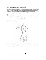
Here is the electrical circuit diagram for the sensor
1
C1
10k 25C
b
RT1
Off Board
T
10.0k
R1
0.1
C2
ADC
Figure 1
The thermistor (RT1) is connected to the positive supply. The positions of RT1 and R1 could have as easily been reversed and
RT1 connected to the negative supply, but the positive connection has the advantage of producing an output voltage that
increases with temperature. Also, if the Analog to Digital Converter (ADC) has a fairly consistent input impedance, its effect on
R1 can be included as a simple parallel sum.
The parameters given for RT1 (Β = 3750 and R0 = 10k Ohms) are the manufacture’s typical values. There are usually several
tolerance grades available with ±10% being the least expensive. 5% tolerance units are very common, while 1% or better units
begin to cost a lot more. The repeatability of a given unit is usually very good. Even a unit with a 10% manufacturing tolerance
can be calibrated to measure with an accuracy better than 0.1°C over a wide temperature range. The long term stability of a
thermistor sensor is usually determined by the packaging. Hermetic glass bead packages have good long term stability, as do
some glasscoated surface mount units.
Referring to Fig.1, capacitor C2 is a radio frequency interference filter. C2 may not be required for many applications. Capacitor
C1 acts as a low pass filter, it not only reduces high frequency noise, it also reduces errors due to ADC charge injection. For
many applications C1 could be reduced or eliminated. The thermistor’s own thermal time constant is often several seconds,
which tends to be the limiting factor on signal bandwidth.
Selecting the value of R1 is an interesting problem. Different values for R1 produce different curvatures in the circuit’s temperature
to voltage relationship. For temperature controllers operating at a fixed temperature, R1 is usually selected to give the
greatest sensitivity at the operating temperature. For measuring instruments, like this one, a common choice is to pick R1 so that
the sensitivity is equal at the extremes of the measurement range. This constraint is easy to express analytically, and it tends to
reduce the nonlinearity of the voltage vs temperature relationship over the range of interest.

Selecting the value of R1 is an interesting problem. Different values for R1 produce different curvatures in the circuit’s tempera-
4 ture to voltage relationship. For temperature controllers operating at a fixed temperature, R1 is usually selected Thermistors
to give the
greatest sensitivity at the operating temperature. For measuring instruments, like this one, a common choice is to pick R1 so that
the sensitivity is equal at the extremes of the measurement range. This constraint is easy to express analytically, and it tends to
reduce the nonlinearity of the voltage vs temperature relationship over the range of interest.
To analyze this more precisely, begin with the voltage to thermistor resistance relationship for the circuit in Fig.1
v 1
1 r1
The lowercase "v" in the equation is the voltage ratio between the ADC input voltage and the positive supply voltage, v is
always between zero and one. "r1" is the resistance ratio of the thermistor RT1 to the fixed resistor R1, r1 may be any nonzero
positive real number, but it usually lies between 1000 and 1/1000.
Using equation (1), the ratio of thermistor resistance at a given temperature to resistance at the reference temperature (r) is
Ln r Ln R
Β
R0
1
T 1
T0
Putting (10) into (9) and manipulating gets
v
1
1
Β
1 s T
1
T
0
The symbol (s) has been introduced for the ratio R0 / R1
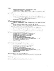
Equation (11) has been plotted for various values of (s) in Fig.2.
1
0.8
0.6
0.4
0.2
v
v versus T for various values of s
260 280 300 320 340
T ° K
Figure 2
In Fig.2 The red lines cover the range of (s) from 0.1 to 1, the green lines cover (s) from 2 to 10 and the blue lines cover (s)
equal 20 to 100.
(9)
(10)
(11)

Thermistors 5
Intuitively, the best choice for R1 is the one that results in the (v) vs (T) graph that is closest to a 45° diagonal line over the
temperature range of interest. This can be approximated analytically by using the equalslope concept mentioned before.
From (11) the slope of the graph is found to be
v
T
1
Β
s Β T
1
T0
1
T
Β
s T T
1
T0
2
Setting the slopes equal at the temperature extremes (TH ) and (TL ) produces a formula for the ‘optimal’ (s)
Β
2 T
H T
s T H 2 T
L TL 0
Β
Β
2 T
H TH
Β
Β
2 T L T L
For the example at hand, equation (13) suggests setting R1 = 7417 Ohms. The value actually chosen for R1 in Fig.1 was 10k
Ohms. 10k is simply a more convenient value. Also, eyeballing Fig.2, it looks like 10k might be a better choice, even if it isn’t,
it’s close enough.
So far in this example, we have relied exclusively on the simplified model. It would be nice to know the magnitude of the errors
being introduced by using the simple model. To investigate that we need to compare the simplified model to the real thermistor
behavior. For theoretical purposes this can be done by comparing the simplified model to the full cubic approximation because
we know from experience that the cubic model is very accurate.
Here is some data from thermistor measurements
Temperature °C r
292 0.0025
255 0.004
240 0.0045
195 0.01
160 0.02
120 0.05
70 0.2
50 0.4
37 20
60 100
Table 1
In Table 1 the left column is the thermistor’s temperature (T) in °C, the right column is the thermistor’s resistance ratio (r) which
is the ratio of resistance at temperature (T) to the resistance at the reference temperature (T0 ).
Fitting the data in Table 1 to equation (3) by the method of least squares produces the following "truth" model
Ln r 14.0094 4975.08
T
300985
T2 1.81688 107
T3 Equation (14) is a truth model in that we assume that it accurately indicates the behavior of the real system. It does not account
for various effects such as self heating or time varying behavior, nor should it for our current purposes.
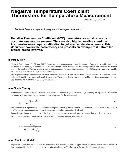
As a confidence building measure it’s a good idea to graph equation (14) along with the data from Table 1
(12)
(13)
(14)

6 Thermistors
100
10
1
0.1
0.01
r
truth model of a real thermistor
250 300 350 400 450 500 550
Figure 3
As the graph shows, equation (14) agrees quite well with the actual data.
T ° K
To properly compare the truth model to the simplified model, we must fit the simplified model to the truth model. This is
because so far the simplified model has relied on the manufacture’s nominal values for it’s parameters, as a result most of the
error between the simplified model so far and the truth model would be the result of miscalibration. By fitting the simple model
to the truth model, we effectively will calibrate the simple model, thus isolating the calibration error from the modeling error.
Performing a least squares fit to the truth model over the application temperature range at 1°C intervals yields this simplified
model
Ln r 3536.95
1 1
T 297.134
To calculate the error introduced by (15), we first assume that the true temperature is known, we then use (14) to calculate the
resulting true resistance ratio, we then invert (15) to find the temperature indicated by the simplified model. Finally we subtract
the true temperature to get the temperature error. The resulting error plot is shown in the next figure.
(15)

Thermistors 7
Error° K
1.25
1
0.75
0.5
0.25
-0.25
Error plot for the simplified model
260 280 300 320 340
T ° K
Figure 4
As the figure shows, the maximum error from the simplified model in our example is about 1.25°C, the RMS error is probably
closer to 1/2°C.
For comparison let’s look at the full model without the squared term, namely
Ln r A B
T D
T3 Fitting this model to our truth model yields
Ln r 12.7839 3918.51 1.01646 107
T
T3 The error plot for the squareless model is given in the next figure
(16)
(17)

8 Thermistors
Error° K
0.1
0.05
-0.05
Error plot for the squareless model
260 280 300 320 340
T ° K
Figure 5
As the figure shows, the error introduced into our example by dropping the squared term is typically less than 0.1°C . For many
applications this would be acceptable.
Even the simplified model requires taking a logarithm to find the temperature. For certain applications, such as those restricted
to integer math on a microcontroller, this is undesirable. If the accuracy requirements aren’t too high, the logarithm can be
avoided with a polynomial approximation.
The true temperature vs voltage equation for our example can be found by combining (9) with (3) it is
1
1 s r 1 s Exp A
v B
T C D
T2 T3 Setting (s)=1, and graphing
(18)

Thermistors 9
T ° K
340
320
300
280
260
Truth model for Temperature vs Voltage
0.2 0.4 0.6 0.8
Normalized
voltage
Figure 6
As the figure shows, the temperature voltage relationship is approximately linear with a possibly cubic nonlinearity. Fitting 500
samples of this curve to a cubic polynomial by the least square method results in this equation
T 227.929 251.624 v 358.996 v 2 267.536 v 3
Fig.7 shows the error plot for equation (19) combined with Fig.4, the error plot for the simplified equation
(19)

10 Thermistors
Error ° K
2
1.5
1
0.5
-0.5
-1
Error plot for the cubic polynomial and
simplified exponential models
exponential model in Blue
260 280 300 320 340
T ° K
Figure 7
Fig.7 shows the error graphs for both the current cubic polynomial model and the old simplified exponential model. The error
introduced using the cubic approximation is about the same as that of the simplified model except at the extremes of the temperature
range. This is pretty good if you’re stuck with integer math, considering that the cubic approximation requires only 3
multiplies.
It should be noted that the use of the polynomial model introduces some complications. The simplified exponential model only
requires the parameters (R0 ) and (Β), which are usually available from the manufacture’s data sheet. The polynomial model
requires a least squares fit, ideally to real thermistor data, which requires several measurements. Although the polynomial model
can be fit to the simplified exponential model calculated from the manufacture’s data, doing so will introduce the errors from the
simplified model into the polynomial. These errors will add in a statistical fashion with the inherent polynomial modeling errors,
generally reducing the accuracy of the polynomial model compared to the simplified exponential model calculated directly from
the manufacture’s data. The only way around this is to perform calibration measurements.
To summarize the results of the error analysis so far. The truth model is reported to be accurate to within 1/100°C over a fairly
wide temperature range. The model with the square term suppressed is probably good to within 1/10°C over spans exceeding
100°C and requires a minimum of 3 calibration points. The simplified exponential model is accurate to about 1°C over a 100°C
span. The cubic polynomial model has an accuracy comparable to the simplified exponential model.
Calibration
Most commercial thermistors are specified at 25°C to have a specific resistance, and a characteristic Β . Typical tolerances for
inexpensive parts are R0 ± 5% and Β ± 2%. To see the effects of thermistor error tolerance on measurement accuracy, we will
create an error plot using the nominal simplified exponential model as the truth model and plot the difference as each parameter
is varied to its maximum tolerance.

Thermistors 11
R5%
R5%
Β2%
Β2%
Error ° K
1.5
1
0.5
-0.5
-1
-1.5
Error plot for the simplified model
Showing the effects of manufacturing tolerance
260 280 300 320 340
T ° K
Figure 8
Fig.8 displays the effect of ±5% error in reference resistance, and ±2% error in the Β factor on temperature measurement accuracy
for our example problem. The figure shows that an error in Β, by definition, only manifests itself away from the reference
temperature. The system as a whole is nonlinear, but for reasonably tight tolerances the effect of varying tolerance will be
proportional to that shown in Fig.8. Both miscalibrations contribute about 1°C of error, more at the extremes, particularly at high
temperature, so the total miscalibration error can be greater than 2°C. To correct for miscalibrated resistance requires one
measurement. Complete calibration of the simple model requires only two measurements, but more measurements have the
potential to improve the accuracy slightly.
When calibrating with only a few points it is best to choose points of interest to the application. For high volume or high accuracy
work involving many calibration points it may be worthwhile to set up an automated calibration sweep procedure. This is
easier than arranging for many different constant temperatures, and much faster in operation.
Summary
Thermistors, while nonlinear, can be accurately modeled.
Models with reduced complexity are available
Thermistors are subject to selfheating effects
Choice of companion resistor in the thermistor voltage divider circuit depends on the application and on the temperature measurement
range
The final accuracy of a thermistor sensor depends mostly on the quality of the calibration and modeling used
Thermistor Model Typical Error for 100°C range Calibrations Required
Third Order Polynomial with Exponential 0.01 °C 4
ThirdOrder Exponential with Square Term Removed 0.1 °C 3
Simple Exponential 1 °C 02
Third Order Polynomial 12 °C 03
Table 2
Over an approximately 100°C span, a 5% resistance tolerance contributes to ±1°C of measurement error. A 2% tolerance in the Β
factor also contributes about 1°C of error. In the worst case, all listed errors must be added together to find the maximum error
due to the thermistor system. For some applications statistical considerations may indicate a lower error growth rate. More

12 Thermistors
Over an approximately 100°C span, a 5% resistance tolerance contributes to ±1°C of measurement error. A 2% tolerance in the Β
factor also contributes about 1°C of error. In the worst case, all listed errors must be added together to find the maximum error
due to the thermistor system. For some applications statistical considerations may indicate a lower error growth rate. More
sophisticated analysis will usually yield more sophisticated results.