Computational Hydraulics (Web) - E - nptel

Computational Hydraulics
Prof. M.S.Mohan Kumar
Department of Civil Engineering

Introduction to Hydraulics
of Open Channels
Module 1
3 lectures

Basic Basic Concepts Concepts
Topics to be covered
Conservation Laws Laws
Critical Critical Flows Flows
Uniform Uniform Flows Flows
Gradually Gradually Varied Varied Flows Flows
Rapidly Rapidly Varied Varied Flows Flows
Unsteady Unsteady Flows
Flows

Basic Concepts
Open Channel flows deal with flow of water in open channels
Pressure is atmospheric at the water surface and the
pressure is equal to the depth of water at any section
Pressure head is the ratio of pressure and the specific weight
of water
Elevation head or the datum head is the height of the
section under consideration above a datum
Velocity head (= (=vv 22 /2g) /2g)
is due to the average velocity of flow
in that vertical section

Basic Concepts Cont… Cont
Total head = =p/ p/γγ + + vv 22 /2g /2g + + zz
Pressure head = p/γγ p/
Velocity head = =vv 22 /2g /2g
Datum head = zz
The The flow of water in an open channel is mainly due to head
gradient and gravity
Open Open Channels are mainly used to transport water for
irrigation, industry and domestic water supply

Conservation Laws
The The main main conservation conservation laws laws used used in in open open channels channels are are
Conservation Laws
Conservation of Mass
Conservation of Momentum
Conservation of Energy

Conservation of Mass
Conservation of of Mass Mass
In In any any control control volume volume consisting consisting of of the the fluid fluid ( ( water) water) under under
consideration, consideration, the the net net change change of of mass mass in in the the control control volume volume
due due to to inflow inflow and and out out flow flow is is equal equal to to the the the the net net rate rate of of
change change of of mass mass in in the the control control volume volume
This This leads to the classical continuity equation balancing the
inflow, out flow and the storage change in the control
volume.
Since Since we are considering only water which is treated as
incompressible, the density effect can be ignored

Conservation of Momentum and energy
Conservation of of Momentum
Momentum
This This law law states states that that the the rate rate of of change change of of momentum momentum in in the the
control control volume volume is is equal equal to to the the net net forces forces acting acting on on the the
control control volume volume
Since Since the water under consideration is moving, it is acted
upon by external forces
Essentially Essentially this leads to the Newton’s Newton s second law
Conservation of of Energy Energy
This This law law states states that that neither neither the the energy energy can can be be created created or or
destroyed. destroyed. It It only only changes changes its its form.
form.

Conservation of Energy
Mainly Mainly in open channels the energy will be in the form of potential potential
energy
and kinetic energy
Potential Potential energy is due to the elevation of the water parcel while while
the
kinetic energy is due to its movement
In In the context of open channel flow the total energy due these factors factors
between any two sections is conserved
This This conservation of energy principle leads to the classical Bernoulli Bernoulli’s
s
equation
P/γ P/ + + vv 22 /2g /2g + + z z = = Constant Constant
When When used between two sections this equation has to account for the
energy loss between the two sections which is due to the resistance resistance
to the
flow by the bed shear etc.

Types of Open Channel Flows
Depending Depending on on the the Froude Froude number number (F (Frr))
the the flow flow in in an an open open
channel channel is is classified classified as as Sub Sub critical critical flow, flow, Super Super Critical Critical
flow, flow, and and Critical Critical flow, flow, where where Froude Froude number number can can be be defined defined
as as V
F r =
gy
Open channel flow
Sub-critical Sub critical flow Critical flow Super critical flow
Fr 1

Types of Open Channel Flow Cont...
Open Channel Flow
Unsteady Steady
Varied Uniform Varied
Gradually
Rapidly
Gradually
Rapidly

Types of Open Channel Flow Cont… Cont
Steady Steady Flow Flow
Flow is said to be steady when discharge does not
change along the course of the channel flow
Unsteady Unsteady Flow Flow
Flow is said to be unsteady when the discharge
changes with time
Uniform Uniform Flow Flow
Flow is said to be uniform when both the depth and
discharge is same at any two sections of the channel

Types of Open Channel Cont… Cont
Gradually Gradually Varied Varied Flow Flow
Flow is said to be gradually varied when ever the
depth changes gradually along the channel
Rapidly Rapidly varied varied flow flow
Whenever the flow depth changes rapidly along the
channel the flow is termed rapidly varied flow
Spatially Spatially varied varied flow flow
Whenever the depth of flow changes gradually due
to change in discharge the flow is termed spatially
varied flow

Types of Open Channel Flow cont… cont
Unsteady Unsteady Flow Flow
Whenever the discharge and depth of flow changes
with time, the flow is termed unsteady flow
Types of possible flow
Steady uniform flow Steady non-uniform non uniform flow Unsteady non-uniform non uniform flow
kinematic wave diffusion wave
dynamic wave

Specific Specific Energy Energy
Definitions
It It is is defined defined as as the the energy energy acquired acquired by by the the water water at at a a
section section due due to to its its depth depth and and the the velocity velocity with with which which it it
is is flowing flowing
Specific Specific Energy E is given by, E E = = y y + + vv 22 /2g /2g
Where y is the depth of flow at that section
and v is the average velocity of flow
Specific Specific energy is minimum at critical
condition

Specific Specific Force Force
Definitions
It It is is defined defined as as the the sum sum of of the the momentum momentum of of the the flow flow passing passing
through through the the channel channel section section per per unit unit time time per per unit unit weight weight of of
water water and and the the force force per per unit unit weight weight of of water water
F F = = QQ 22 /gA /gA +yA + yA
The specific forces of two sections are equal
provided that the external forces and the weight
effect of water in the reach between the two
sections can be ignored.
At the critical state of flow the specific force is a
minimum for the given discharge.

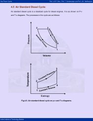
Critical Flow
Flow Flow is is critical critical when when the the specific specific energy energy is is minimum. minimum.
Also Also whenever whenever the the flow flow changes changes from from sub sub critical critical to to
super super critical critical or or vice vice versa versa the the flow flow has has to to go go
through through critical critical condition condition
figure figure is is shown shown in in next next slide slide
Sub Sub-critical critical flow-the flow the depth of flow will be higher
whereas the velocity will be lower.
Super Super-critical critical flow-the flow the depth of flow will be lower
but the velocity will be higher
Critical Critical flow: flow:
Flow over a free over-fall over fall

Depth of water Surface (y)
45°
Specific energy diagram
Emin
Critical Depth
y c
C
E=y
1
2
Specific Energy (E)
y
E-y curve
y
Specific Energy Curve for a given discharge
1
2
Alternate Depths

Characteristics of Critical Flow
Specific Specific Energy ( (E E = = y+Q y+Q22
/2gA /2gA22
) is minimum
For For Specific energy to be a minimum dE/dy dE/dy = = 00
dE
dy
2
Q
= 1−
3
gA
However, However, dA==Tdy dA Tdy, , where T is the width of the
channel at the water surface, then applying dE/dy dE/dy = =
0, 0, will will result result in in following following
Q
2
c
3
c
gA
T
= 1
A c
=
T
c
Q
gA
2
2
c
⋅
dA
dy
Ac VC
=
T g
c
2

Characteristics of Critical Flow
For a rectangular channel AA c c //TT cc==yy cc
Following the derivation for a rectangular channel,
F
r
=
The same principle is valid for trapezoidal and other
cross sections
V
Critical flow condition defines an unique relationship
between depth and discharge which is very useful in the
design of flow measurement structures
c
gy
c
= 1

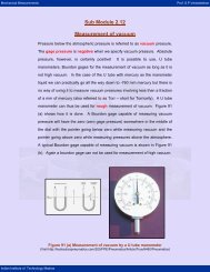
Uniform Flows
This This is one of the most important concept in open channel
flows
The The most important equation for uniform flow is Manning’s Manning s
equation given by
1
V = R
n
Where RR = the hydraulic radius = A/P A/P
PP = wetted perimeter = f(y, f(y, SS 00))
YY = depth of the channel bed
SS 00 = bed slope (same as the energy slope, SS ff) )
n n = the Manning’s Manning s dimensional empirical constant
2/
3
S
1/
2

V12/2g
y1
z1
1
Uniform Flows
So 1
Energy Grade Line
Control Volume
Datum
Steady Uniform Flow in an Open Channel
1
Sf
2
hf
v22/2g
z2 y2

Uniform Flow
Example Example : Flow in an open channel
This This concept is used in most of the open channel flow design
The The uniform flow means that there is no acceleration to the
flow leading to the weight component of the flow being
balanced by the resistance offered by the bed shear
In In terms of discharge the Manning’s Manning s equation is given by
1
Q =
n
AR
2/
3
S
1/
2

Uniform Flow
This This is a non linear equation in y the depth of flow for which
most of the computations will be made
Derivation Derivation of uniform flow equation is given below, where
W
sinθ
= weight component of the fluid mass in the
direction of flow
τ 0
P∆x
= bed shear stress
= surface area of the channel

Uniform Flow
The force balance equation can be written as
Or
Or
W sinθ −τ 0 P∆x
=
γA∆xsinθ
−τ
0 P∆x
=
A
τ 0 = γ sinθ
P
Now A/P A/P is the hydraulic radius, RR, , and sinθθ sin is
the slope of the channel
the slope of the channel SS 00
0
0

Uniform Flow
The shear stress can be expressed as
Where cc ff is resistance coefficient, VV is the mean
velocity ρρ is the mass density
Therefore the previous equation can be written as
Or
c f
τ =
where CC is Chezy’s Chezy constant
For Manning’s Manning s equation
0
c f ρ
( 2
V / 2)
2
V
2g
ρ = γRS
V = RS
0
0 = C RS0
2
c f
1.
49
C =
R
n
1/
6

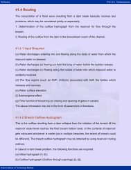
Gradually Varied Flow
Flow Flow is is said said to to be be gradually gradually varied varied whenever whenever the the depth depth of of
flow flow changed changed gradually gradually
The The governing equation for gradually varied flow is given by
dy
dx
=
2
1− Fr
Where Where the variation of depth y y with the channel distance xx
is shown to be a function of bed slope SS 00, , Friction Slope SS ff
and the flow Froude number FF rr. .
This This is a non linear equation with the depth varying as a
non linear function
S
0
−
S
f

Gradually Varied Flow
Energy-grade line (slope = Sf)
z y v2/2g
Water surface (slope = Sw)
Channel bottom (slope = So)
Datum
Total head at a channel section

Gradually Varied Flow
Derivation of gradually varied flow is as follows… follows
The conservation of energy at two sections of a
reach of length ∆∆xx, , can be written as
V1
V2
y1 + + S0∆x
= y2
+ + S f ∆x
2g
2g
Now, let and
2
∆y
= y −
Then the above equation becomes
2
y
1
2
d ⎛V
⎞
∆y
= S ∆x
− S f ∆x
− ∆x
dx ⎜
g ⎟
0
⎝ 2 ⎠
2
V
2
2
2g
2
V1
−
2g
=
d
dx
2 ⎛V
⎞
⎜ ∆x
g ⎟
⎝ 2 ⎠

Gradually Varied Flow
Dividing through ∆∆xx and taking the limit as ∆∆xx
approaches zero gives us
dy
dx
After simplification,
dx
2
d ⎛V
⎞
+ = S
dx ⎜
g ⎟ 0
⎝ 2 ⎠
S
=
1+
d
Further simplification can be done in terms of
Froude number
−
S
dy 0 f
d
dy
−
S
( 2
V / 2g
) / dy
2
2
⎛V
⎞ d ⎛ Q
⎜
⎟ = ⎜
⎝ 2g ⎠ dy ⎝ 2gA
f
2
⎞
⎟
⎠

Gradually Varied Flow
After differentiating the right side of the previous
equation,
d
dy
2 ⎛V
⎞
⎜
g ⎟
⎝ 2 ⎠
− 2Q
2gA
But dA/dy=T, dA/dy=T,
and and A/T=D, A/T=D, therefore,
d
dy
2 ⎛V
⎞
⎜
2g
⎟
⎝ ⎠
Finally the general differential equation can be
written as
dy
dx
=
=
=
S
− Q
gA
0
−
2
2
D
S
2
1− Fr
3
f
2
⋅
dA
dy
= −F
2
r

Gradually Varied Flow
Numerical Numerical integration of the gradually varied flow equation
will give the water surface profile along the channel
Depending Depending on the depth of flow where it lies when compared
with the normal depth and the critical depth along with the
bed slope compared with the friction slope different types of
profiles are formed such as M (mild), C (critical), S (steep)
profiles. All these have real examples.
M M (mild)-If (mild) If the slope is so small that the normal depth
(Uniform flow depth) is greater than critical depth for the
given discharge, then the slope of the channel is mild.
mild

Gradually Varied Flow
C (critical)-if (critical) if the slope’s slope s normal depth equals its critical
depth, then we call it a critical slope, denoted by C
S (steep)-if (steep) if the channel slope is so steep that a normal
depth less than critical is produced, then the channel is
steep, steep,
and water surface profile designated as S

Rapidly Varied Flow
This flow has very pronounced curvature of the streamlines
It is such that pressure distribution cannot be assumed to
be hydrostatic
The rapid variation in flow regime often take place in short
span
When rapidly varied flow occurs in a sudden-transition
sudden transition
structure, the physical characteristics of the flow are
basically fixed by the boundary geometry of the structure as
well as by the state of the flow
Examples:
Channel expansion and cannel contraction
Sharp crested weirs
Broad crested weirs

Unsteady flows
When the flow conditions vary with respect to time, we call
it unsteady flows.
Some terminologies used for the analysis of unsteady flows
are defined below:
Wave:: Wave it is defined as a temporal or spatial variation of flow
depth and rate of discharge.
Wave Wave length: length:
it is the distance between two adjacent wave
crests or trough
Amplitude: Amplitude:
it is the height between the maximum water
level and the still water level

Unsteady flows definitions
Wave Wave celerity celerity (c): (c): relative velocity of a wave with respect
to fluid in which it is flowing with VV
Absolute Absolute wave wave velocity velocity (VV ( ww): ): velocity with respect to
fixed reference as given below
V w
=
Plus sign if the wave is traveling in the flow direction and
minus for if the wave is traveling in the direction opposite to
flow
For shallow water waves c =
gy0
where yy 00=undisturbed
=undisturbed
flow depth.
V
±
c

Unsteady flows examples
Unsteady Unsteady flows flows occur occur due due to to following following reasons: reasons:
1. Surges in power canals or tunnels
2. Surges in upstream or downstream channels produced by
starting or stopping of pumps and opening and closing of
control gates
3. Waves in navigation channels produced by the operation of
navigation locks
4. Flood waves in streams, rivers, and drainage channels due
to rainstorms and snowmelt
5. Tides in estuaries, bays and inlets

Unsteady flows
Unsteady flow commonly encountered in an open channels
and deals with translatory waves. Translatory waves is a
gravity wave that propagates in an open channel and
results in appreciable displacement of the water particles in
a direction parallel to the flow
For purpose of analytical discussion, unsteady flow is
classified into two types, namely, gradually varied and
rapidly varied unsteady flow
In gradually varied flow the curvature of the wave profile is
mild, and the change in depth is gradual
In the rapidly varied flow the curvature of the wave profile
is very large and so the surface of the profile may become
virtually discontinuous.

Unsteady flows cont… cont
Continuity equation for unsteady flow in an open
channel
∂V
D
∂x
+ V
∂y
∂x
For a rectangular channel of infinite width, may be
written
∂q
∂x
+
∂t
When the channel is to feed laterally with a
supplementary discharge of q’ q per unit length, for
instance, into an area that is being flooded over a
dike
+
∂y
∂y
∂t
=
0
=
0

The equation
Unsteady flows cont… cont
∂Q
∂x
+
∂A
∂t
'
+ q = 0
The general dynamic equation for gradually
varied unsteady flow is given by:
∂y
αV
+
∂x
g
∂V
∂x
+
1
g
∂V
∂t
'
=
0

Review of Hydraulics of
Pipe Flows
Module2
3 lectures

General General introduction
introduction
Energy Energy equation equation
Head Head loss loss equations equations
Contents
Head Head discharge discharge relationships
Pipe Pipe transients transients flows flows through through
pipe pipe networks networks
Solving Solving pipe pipe network network problems
problems

General Introduction
Pipe flows are mainly due to pressure difference between
two sections
Here also the total head is made up of pressure head, datum
head and velocity head
The principle of continuity, energy, momentum is also used
in this type of flow.
For example, to design a pipe, we use the continuity and
energy equations to obtain the required pipe diameter
Then applying the momentum equation, we get the forces
acting on bends for a given discharge

General introduction
In the design and operation of a pipeline, the main
considerations are head losses, forces and stresses
acting on the pipe material, and discharge.
Head loss for a given discharge relates to flow
efficiency; i.e an optimum size of pipe will yield the
least overall cost of installation and operation for
the desired discharge.
Choosing a small pipe results in low initial costs,
however, subsequent costs may be excessively
large because of high energy cost from large head
losses

Energy equation
The design of conduit should be such that it needs least
cost for a given discharge
The hydraulic aspect of the problem require applying the
one dimensional steady flow form of the energy equation:
p
γ
1
2
2
V
p V
+ α 1 + z + hp
= 2 + 2
1 1
α2
+ z2
2g
2g
Where p/γγ p/ =pressure head
ααVV 22 /2g /2g =velocity head
z z =elevation head
hh pp=head =head supplied by a pump
hh t t =head supplied to a turbine
=head loss between 1 and 2
hh LL =head loss between 1 and 2
γ
+
h
t
+
h
L

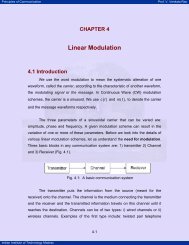
Energy equation
z1
hp
Pump
Energy Grade Line
Hydraulic Grade Line
The Schematic representation of the energy equation
p/y
z
v2/2g
z = 0 Datum
z2

Velocity Velocity head head
Energy equation
In ααVV 22 /2g, /2g,
the velocity VV is the mean velocity in the
conduit at a given section and is obtained by
V=Q/A, V=Q/A,
where QQ is the discharge, and AA is the
cross-sectional cross sectional area of the conduit.
The kinetic energy correction factor is given by α, ,
and it is defines as, where uu=velocity =velocity at any point
in the section
3
α
=
∫ u dA
A
3
V A
α has minimum value of unity when the velocity is
uniform across the section

Energy equation cont… cont
Velocity Velocity head head cont…… cont
α has values greater than unity depending on the degree of
velocity variation across a section
For laminar flow in a pipe, velocity distribution is parabolic
across the section of the pipe, and α has value of 2.0
However, if the flow is turbulent, as is the usual case for
water flow through the large conduits, the velocity is fairly
uniform over most of the conduit section, and α has value
near unity (typically: 1.04< α < 1.06).
Therefore, in hydraulic engineering for ease of application
in pipe flow, the value of α is usually assumed to be unity,
and the velocity head is then simply VV 22 /2g.
/2g

Energy equation cont… cont
Pump Pump or or turbine turbine head head
The head supplied by a pump is directly
related to the power supplied to the flow as
given below
P = Qγh
Likewise if head is supplied to turbine, the
power supplied to the turbine will be
P =
Qγh
These two equations represents the power
supplied directly or power taken out directly
from the flow
p
t

Energy equation cont… cont
Head--loss Head loss term term
The head loss term hh LL accounts for the conversion
of mechanical energy to internal energy (heat),
when this conversion occurs, the internal energy is
not readily converted back to useful mechanical
energy, therefore it is called head head loss loss
Head loss results from viscous resistance to flow
(friction) at the conduit wall or from the viscous
dissipation of turbulence usually occurring with
separated flow, such as in bends, fittings or outlet
works.

Head loss calculation
Head loss is due to friction between the fluid and
the pipe wall and turbulence within the fluid
The rate of head loss depend on roughness
element size apart from velocity and pipe diameter
Further the head loss also depends on whether the
pipe is hydraulically smooth, rough or somewhere
in between
In water distribution system , head loss is also due
to bends, valves and changes in pipe diameter

Head loss calculation
Head loss for steady flow through a straight pipe:
τ
∆ p
τ
h
0
0
Aw = ∆ pA r
=
=
=
4 L τ
fρ
V
∆ p
γ
This is known as Darcy-Weisbach
Darcy Weisbach equation
=
0
2
f
h/L=S, h/L=S,
is slope of the hydraulic and energy grade
lines for a pipe of constant diameter
/
/
D
8
L
D
V
2
2 g

Head Head loss loss in in laminar laminar flow: flow:
Head loss calculation
Hagen-Poiseuille
Hagen Poiseuille equation gives
Combining above with Darcy-Weisbach
Darcy Weisbach equation, gives f
Also we can write in terms of Reynolds number
This relation is valid for NN rr

Head loss calculation
Head Head loss loss in in turbulent turbulent flow: flow:
In turbulent flow, the friction factor is a function of both
Reynolds number and pipe roughness
As the roughness size or the velocity increases, flow is
wholly rough and f depends on the relative roughness
Where graphical determination of the friction factor is
acceptable, it is possible to use a Moody diagram.
This diagram gives the friction factor over a wide range of
Reynolds numbers for laminar flow and smooth, transition,
and rough turbulent flow

Head loss calculation
The quantities shown in Moody Diagram are dimensionless
so they can be used with any system of units
Moody’s Moody s diagram can be followed from any reference book
MINOR MINOR LOSSES LOSSES
Energy losses caused by valves, bends and changes in pipe
diameter
This is smaller than friction losses in straight sections of
pipe and for all practical purposes ignored
Minor losses are significant in valves and fittings, which
creates turbulence in excess of that produced in a straight
pipe

Head loss calculation
Minor losses can be expressed in three ways:
1. A minor loss coefficient K may be used to give
head loss as a function of velocity head,
h
=
K
V
2g
2. Minor losses may be expressed in terms of the
equivalent length of straight pipe, or as pipe
diameters (L/D) which produces the same head
loss.
h =
f
2
L
D
V
2
2g

Head loss calculation
1. A flow coefficient Cv which gives a flow that will
pass through the valve at a pressure drop of
1psi may be specified. Given the flow coefficient
the head loss can be calculated as
h
18.
5
× 10
C
The flow coefficient can be related to the minor loss
coefficient by
K
=
=
18.
5
6
v 2
2
× 10
C
2
v
6
D
g
D
4
2
V
2

Energy Equation for Flow in pipes
Energy equation for pipe flow
2
2
P1
V1
P2
V2
z 1 + + = z2
+ + +
ρg
2g
ρg
2g
The energy equation represents elevation, pressure, and velocity forms
of energy. The energy equation for a fluid moving in a closed conduit is
written between two locations at a distance (length) L apart. Energy
losses for flow through ducts and pipes consist of major losses and
minor losses. losses
Minor Loss Calculations for Fluid Flow
h m
2
V
=
K
2g
Minor losses are due to fittings such as valves and elbows
hL

Major Loss Calculation for Fluid Flow
Using Darcy-Weisbach
Darcy Weisbach Friction Loss Equation
Major losses are due to friction between the moving fluid
and the inside walls of the duct.
The Darcy-Weisbach
Darcy Weisbach method is generally considered more
accurate than the Hazen-Williams Hazen Williams method. Additionally,
the Darcy-Weisbach
Darcy Weisbach method is valid for any liquid or gas.
Moody Friction Factor Calculator

Major Loss Calculation in pipes
Using Hazen-Williams Hazen Williams Friction Loss Equation
Hazen-Williams Hazen Williams is only valid for water at ordinary
temperatures (40 to 75 oF). F). The Hazen-Williams Hazen Williams method is
very popular, especially among civil engineers, since its
friction coefficient (C) is not a function of velocity or duct
(pipe) diameter. Hazen-Williams Hazen Williams is simpler than Darcy- Darcy
Weisbach for calculations where one can solve for flow-
rate, velocity, or diameter

Transient flow through long pipes
Intermediate flow while changing from one
steady state to another is called transient
flow
This occurs due to design or operating
errors or equipment malfunction.
This transient state pressure causes lots of
damage to the network system
Pressure rise in a close conduit caused by an
instantaneous change in flow velocity

Transient flow through long pipes
If the flow velocity at a point does vary with time, the flow
is unsteady
When the flow conditions are changed from one steady
state to another, the intermediate stage flow is referred to
as transient flow
The terms fluid transients and hydraulic transients are used
in practice
The different flow conditions in a piping system are
discussed as below:

Transient flow through long pipes
Consider a pipe length of length L
Water is flowing from a constant level upstream reservoir
to a valve at downstream
Assume valve is instantaneously closed at time t=t
the full open position to half open position.
t=t00 from
This reduces the flow velocity through the valve, thereby
increasing the pressure at the valve

Transient flow through long pipes
The increased pressure will produce a pressure wave that
will travel back and forth in the pipeline until it is
dissipated because of friction and flow conditions have
become steady again
This time when the flow conditions have become steady
again, let us call it t 1.
So the flow regimes can be categorized into
1. Steady flow for t

Transient flow through long pipes
Transient-state Transient state pressures are sometimes reduced to the
vapor pressure of a liquid that results in separating the
liquid column at that section; this is referred to as liquid-
column separation
If the flow conditions are repeated after a fixed time
interval, the flow is called periodic flow, and the time
interval at which the conditions are repeated is called
period
The analysis of transient state conditions in closed conduits
may be classified into two categories: lumped-system
lumped system
approach and distributed system approach

Transient flow through long pipes
In the lumped lumped system system approach the conduit walls
are assumed rigid and the liquid in the conduit is
assumed incompressible, so that it behaves like a
rigid mass, other way flow variables are functions
of time only.
In the distributed distributed system system approach the liquid is
assumed slightly compressible
Therefore flow velocity vary along the length of the
conduit in addition to the variation in time

Transient flow through long pipes
Flow Flow establishment
The 1D form of momentum equation for a control volume
that is fixed in space and does not change shape may be
written as
d
2
2
∑ F = ∫ ρVAdx
+ ( ρAV
) out −(
ρAV
)
dt
If the liquid is assumed incompressible and the pipe is rigid,
then at any instant the velocity along the pipe will be same,
2
( ρ AV ) =
( ρAV
)
in
2
out
in

Transient flow through long pipes
Substituting for all the forces acting on the control
volume
d
pA +
γ AL sin α − τ 0πDL = ( VρAL)
dt
Where
p p =γ(h = (h--VV 22 /2g) /2g)
α=pipe =pipe slope slope
D=pipe D=pipe diameter diameter
L=pipe L=pipe length length
γ =specific =specific weight weight of of fluid fluid
τ00=shear =shear stress stress at at the the pipe pipe wall wall

Transient flow through long pipes
Frictional force is replaced by γhh ffAA, , and and HH 00==h+Lsin h+Lsin α and
from Darcy-weisbach
Darcy weisbach friction equation
The resulting equation yields:
fL V V L
H 0 − − = .
D 2g
2g
g
When the flow is fully established, dV/dt=0. dV/dt=0.
The final velocity VV 00 will be such that
2
and hh ff
We use the above relationship to get the time for flow to
establish
dt
2
2
⎡ fL ⎤ V
H 1
0
0 = ⎢ +
D
⎥
⎣ ⎦ 2g
=
2LD
.
D + fL V
2
0
dV
− V
2
dV
dt

Transient flow through long pipes
Change Change in in pressure pressure due due to to rapid rapid flow flow changes changes
When the flow changes are rapid, the fluid
compressibility is needed to taken into account
Changes are not instantaneous throughout the
system, rather pressure waves move back and
forth in the piping system.
Pipe walls to be rigid and the liquid to be slightly
compressible

Transient flows through long pipes
Assume that the flow velocity at the downstream
end is changed from VV to V+∆V, V+ V, thereby changing
the pressure from pp to p+∆pp p+
The change in pressure will produce a pressure
wave that will propagate in the upstream direction
The speed of the wave be a a
The unsteady flow situation can be transformed into
steady flow by assuming the velocity reference
system move with the pressure wave

Transient flows through long pipes
Using momentum equation with control volume approach to
solve for ∆pp
The system is now steady, the momentum equation now
yield
pA − ( p + ∆p)
A = ( V + a + ∆V
)( ρ + ∆ρ)(
V + a + ∆V
) A −
( V
+ a)
ρ(
V + a)
A
By simplifying and discarding terms of higher order, this
equation becomes
2
2
− ∆p
= 2ρV∆V + 2ρ∆Va
+ ∆ρ
V + 2Va
+ a
( )
The general form of the equation for conservation of mass
for one-dimensional one dimensional flows may be written as
x
d
= ∫ ρAdx + −
dt
2
0
x
1
( ρVA)
out ( ρVA)
in

Transient flows through long pipes
For a steady flow first term on the right hand side is zero, then then
we obtain
Simplifying this equation, We have
We may approximate ((V+a V+a)) as a, because V

Introduction to Numerical
Analysis and Its Role in
Computational Hydraulics
Module 3
2 lectures

Contents
Numerical Numerical computing
computing
Computer Computer arithmetic
arithmetic
Parallel Parallel processing
processing
Examples Examples of of problems problems
needing needing numerical numerical
treatment
treatment

What is computational hydraulics?
It is one of the many fields of science in which the
application of computers gives rise to a new way
of working, which is intermediate between purely
theoretical and experimental.
The hydraulics that is reformulated to suit digital
machine processes, is called computational
hydraulics
It is concerned with simulation of the flow of
water, together with its consequences, using
numerical methods on computers

What is computational hydraulics?
There is not a great deal of difference with
computational hydrodynamics or computational
fluid dynamics, but these terms are too much
restricted to the fluid as such.
It seems to be typical of practical problems in
hydraulics that they are rarely directed to the flow
by itself, but rather to some consequences of it,
such as forces on obstacles, transport of heat,
sedimentation of a channel or decay of a pollutant.

Why numerical computing
The higher mathematics can be treated by this method
When there is no analytical solution, numerical analysis
can deal such physical problems
Example: y y = = sin sin (x), (x), has no closed form solution.
The following integral gives the length of one arch of the
above curve
π
∫
2
1
+ cos ( x)
dx
0
Numerical analysis can compute the length of this curve by
standard methods that apply to essentially any integrand
Numerical computing helps in finding effective and efficient
approximations of functions

Why Numerical computing?
linearization of non linear equations
Solves for a large system of linear equations
Deals the ordinary differential equations of any
order and complexity
Numerical solution of Partial differential
equations are of great importance in solving
physical world problems
Solution of initial and boundary value problems
and estimates the eigen values and
eigenvectors.
Fit curves to data by a variety of methods

Computer arithmetic
Numerical method is tedious and repetitive arithmetic,
which is not possible to solve without the help of computer.
On the other hand Numerical analysis is an approximation,
which leads towards some degree of errors
The errors caused by Numerical treatment are defined in
terms of following:
Truncation Truncation error error : the e x can be approximated through
cubic polynomial as shown below
2
x x
p 3 ( x)
= 1 + + +
1!
2!
is an infinitely long series as given below and the error is
due to the truncation of the series
ee xx is an infinitely long series as given below and the error is
e
x
=
p
3
( x)
+
∑ ∞
n=
4
n
x
n!
3
x
3!

• Round
Computer arithmetic
Round--off off error error : digital computers always use floating point
numbers of fixed word length; the true values are not expressed
exactly by such representations. Such error due to this computer
imperfection is round-off round off error.
• Error Error in in original original data data : any physical problem is represented
through mathematical expressions which have some coefficients that that
are imperfectly known.
Blunders : computing machines make mistakes very infrequently,
but since humans are involved in programming, operation, input
preparation, and output interpretation, blunders or gross errors do
occur more frequently than we like to admit.
• Blunders
• Propagated Propagated error error : propagated error is the error caused in the
succeeding steps due to the occurrence of error in the earlier step, step,
such error is in addition to the local errors. If the errors magnified magnified
continuously as the method continues, eventually they will
overshadow the true value, destroying its validity, we call such a
method unstable. unstable.
For stable stable method (which is desired)– desired) errors made
at early points die out as the method continues.

Parallel processing
It is a computing method that can only be
performed on systems containing two or more
processors operating simultaneously. Parallel
processing uses several processors, all working on
different aspects of the same program at the same
time, in order to share the computational load
For extremely large scale problems (short term
weather forecasting, simulation to predict
aerodynamics performance, image processing,
artificial intelligence, multiphase flow in ground
water regime etc), this speeds up the computation
adequately.

Parallel processing
Most computers have just one CPU, but
some models have several. There are even
computers with thousands of CPUs. With
single-CPU single CPU computers, it is possible to
perform parallel processing by connecting
the computers in a network. network.
However, this
type of parallel processing requires very
sophisticated software called distributed
processing software.
Note that parallel processing differs from
multitasking, multitasking,
in which a single CPU executes
several programs at once.

Parallel processing
Types of parallel processing job: In general there are three
types of parallel computing jobs
Parallel Parallel task task
Parametric Parametric sweep sweep
Task Task flow flow
Parallel task
Parallel task
A parallel task can take a number of forms, depending on the
application and the software that supports it. For a
Message Passing Interface (MPI) application, a parallel task
usually consists of a single executable running concurrently
on multiple processors, with communication between the
processes.

Parallel processing
Parametric Parametric Sweep Sweep
A parametric sweep consists of multiple instances of the
same program, usually serial, running concurrently, with
input supplied by an input file and output directed to an
output file. There is no communication or interdependency
among the tasks. Typically, the parallelization is performed
exclusively (or almost exclusively) by the scheduler, based
on the fact that all the tasks are in the same job.
Task Task flow flow
A task flow job is one in which a set of unlike tasks are
executed in a prescribed order, usually because one task
depends on the result of another task.

Introduction to numerical analysis
Any physical problem in hydraulics is represented
through a set of differential equations.
These equations describe the very fundamental
laws of conservation of mass and momentum in
terms of the partial derivatives of dependent
variables.
For any practical purpose we need to know the
values of these variables instead of the values of
their derivatives.

Introduction to numerical analysis
These variables are obtained from integrating those
ODEs/PDEs.
ODEs/PDEs
Because of the presence of nonlinear terms a closed form
solution of these equations is not obtainable, except for
some very simplified cases
Therefore they need to be analyzed numerically, for which
several numerical methods are available
Generally the PDEs we deal in the computational hydraulics
is categorized as elliptic, parabolic and hyperbolic equations

Introduction to numerical analysis
The The following following methods methods have have been been used used for for
numerical numerical integration integration of of the the ODEs ODEs
Euler method
Modified Euler method
Runge-Kutta
Runge Kutta method
Predictor-Corrector Predictor Corrector method

Introduction to numerical analysis
The The following following methods methods have have been been used used for for
numerical numerical integration integration of of the the PDEs PDEs
Characteristics method
Finite difference method
Finite element method
Finite volume method
Spectral method
Boundary element method

Problems needing numerical treatment
Computation of normal depth
Computation of water-surface water surface profiles
Contaminant transport in streams through
an advection-dispersion advection dispersion process
Steady state Ground water flow system
Unsteady state ground water flow system
Flows in pipe network
Computation of kinematic and dynamic
wave equations

Solution of System of
Linear and Non Linear
Equations
Module 4
(4 lectures)

Contents
Set Set of of linear linear equations equations
Matrix Matrix notation notation
Method Method of of
solution:direct and and
iterative iterative
Pathology Pathology of of linear linear
systems systems
Solution Solution of of nonlinear nonlinear
systems systems :Picard : Picard and and
Newton Newton techniques
techniques

Sets of linear equations
Real world problems are presented through a set of
simultaneous equations
F
( x
F
.
.
.
F
1
2
n
1
( x
( x
, x
1
1
, x
, x
,..., x
,..., x
,..., x
Solving a set of simultaneous linear equations needs
several efficient techniques
We need to represent the set of equations through matrix
algebra
2
2
2
n
n
n
)
)
)
=
=
=
0
0
0

Matrix notation
Matrix Matrix : a rectangular array (n x m) of numbers
A =
[ a ]
⎡a
⎢a
⎢
= ⎢ .
⎢ .
⎢ .
⎢
⎣a
11
21
n2
Matrix Addition:
C = A+B = [a [ ij+ ij+
bij] ij]
= [c [ ij], ij],
where
n1
Matrix Multiplication:
AB = C = [a [ ij][b ij][bij]
ij]
= [c [ ij], ij],
where
c
ij
=
m
∑
k = 1
a
ij
ik
b
kj
a
a
a
12
22
.
.
.
.
.
.
.
.
.
a
a
.
.
.
a
1m
2m
nm
⎤
⎥
⎥
⎥
⎥
⎥
⎥
⎦
nxm
c = a +
ij
ij
b
ij
i = 1, 2,...,
n,
j =
1, 2,...,
r.

*AB ≠ BA
kA = = C, C,
where
Matrix notation cont… cont
A A general general relation relation for for Ax Ax = = b b is is
i
No.
ofcols.
b = ∑
k=
1
c ij = kaij
a
ik
x
k
,
i =
1,
2,...,
No.
ofrows

Matrix notation cont… cont
Matrix multiplication gives set of linear equations as:
a11x 11 1+ + a 12x
12 2+…+ a1nx 1n n = b 1, ,
a21x 21 1+ + a 22x
22 2+…+ a2nx 2n n = b 2,
. . .
. . .
. . .
n1x1+ + a n2x
n2 2+…+ ann a n1
nnx n =
= b n,
In simple matrix notation we can write:
Ax = b, where
⎡a11
a12
. . . a1m
⎤
⎢a21
a22
. . . a ⎥
2m
⎢
.
.
⎥
A = ⎢
⎥,
.
⎢ .
.
,
⎥ .
⎢ .
. ⎥ .
⎢
1 2 . . . ⎥
⎣an
an
anm
⎦
2
⎡ x1
⎤
⎢x
⎥
⎢ ⎥
x = ⎢ ⎥
. ,
⎢ ⎥
.
⎢ ⎥
.
⎢⎣
xn
⎥⎦
2
⎡b1
⎤
⎢b
⎥
⎢ ⎥
b
= ⎢ ⎥
⎢ ⎥
⎢ ⎥
⎢⎣
bn
⎥⎦

Matrix notation cont… cont
Diagonal matrix ( only diagonal elements of a
square matrix are nonzero and all off-diagonal
off diagonal
elements are zero)
Identity matrix ( diagonal matrix with all
diagonal elements unity and all off-diagonal
off diagonal
elements are zero)
The order 4 identity matrix is shown below
⎡1
⎢0
⎢0
⎢
⎣0
0
1
0
0
0
0
1
0
0⎤
0⎥
=
0⎥
1⎥
⎦
I4
.

Matrix notation cont… cont
Lower Lower triangular triangular matrix: matrix:
if all the elements above the
diagonal are zero
Upper Upper triangular triangular matrix: matrix:
if all the elements below the
diagonal are zero
Tri--diagonal Tri diagonal matrix: matrix:
if
nonzero elements only on
the diagonal and in the
position adjacent to the
diagonal
T
⎡ ⎤
= ⎢b
d ⎥
⎢
⎣c
e f ⎥
⎦
a
L 0 0 0
U
=
⎡a
⎢0
⎢
⎣0
⎡
⎢c
d
= ⎢ f
⎢
⎢
⎣
b a
0
0 0
0 0
b
d
0
e
g
i
0
0
c ⎤
e ⎥
f ⎥
⎦
⎤
0 0⎥
h 0⎥
j k ⎥
l m
⎥
⎦
0 0

Transpose of a matrix A
(A T ): Rows are written as
columns or vis a versa.
Matrix notation cont… cont
Examples
Determinant of a square
matrix A is given by: ⎥ ⎥
⎡3
−1
4⎤
A = ⎢0
2 − 3
matrix A is given by:
⎢
⎣1
1 2⎦
⎡a
A = ⎢
⎣a
11
21
11
a
a
12
22
22
⎤
⎥
⎦
det( A) =
a a − a a
21
12
T
A
⎡ 3
= ⎢−
1
⎢
⎣ 4
0
2
− 3
1⎤
1⎥
2⎥
⎦

Matrix notation cont… cont
Characteristic Characteristic polynomial polynomial pA (λ) and eigenvalues
eigenvalues
λ of a matrix:
Note: eigenvalues are most important in applied
mathematics
For a square matrix A: we define pA (λ) ) as
pp AA((λλ) ) = = ⏐⏐A A -- λλII⏐⏐ = = det(A det(A -- λλI). I).
If we set pA (λ) ) = 0, solve for the roots, we get
eigenvalues of A
If A is n x n, then pA (λ) ) is polynomial of degree
n
Eigenvector Eigenvector w is a nonzero vector such that
Aw= Aw= λλww, , i.e., (A (A -- λλI)w=0 I)w=0

Methods of solution of set of equations
Direct methods are those that provide the solution in a finite and predeterminable
number of operations using an algorithm that is often
relatively complicated. These methods are useful in linear system of
equations.
Direct Direct methods methods of of solution solution
Gaussian elimination method
4 x
− 3x
x
1
1
1
− 2 x2
+ x
− x2
+ 4 x
− x + 3x
2
= 15
= 8
= 13
Step1: Step1:
Using Matrix notation we can represent the set of equations as
⎡ 4
⎢
⎢−
3
⎢
⎣ 1
−2
− 1
− 1
1⎤
⎥
⎡ x
4⎥
⎢ x
⎥
⎢
3 ⎣ x
⎦
3
3
3
1
2
3
⎤
⎥
⎥
⎦
=
⎡ ⎤
⎢ ⎥
⎢
⎣13⎥
⎦
8
15

Methods of solution cont… cont
Step2: The Augmented coefficient matrix with the right-hand right hand side
vector
Step3: Transform the augmented matrix into Upper triangular form
⎡ 4
⎢−
3
⎢
⎣ 1
Step4: The array in the upper triangular matrix represents the
equations which after Back-substitution Back substitution gives the solution the values
of x 1,x ,x2,x ,x 3
−2
− 1
− 1
1
4
3
AMb
15⎤
8⎥,
13⎥
⎦
2 − 3 → 10 2 R R
⎡ 4
= ⎢−
3
⎢
⎣ 1
⎡
⎢
⎢
⎣
−2
− 1
− 1
3R
( −1)
R
4
0
0
1
1
1
4
3
+ 4R
+ 4R
− −2
10
0
2
3
M
M
M
→
→
15⎤
8⎥
13⎥
⎦
⎡
⎢
⎢
⎣
1
19
− 72
4
0
0
−
−
−2
10
2
15⎤
77⎥
− 216⎥
⎦
1
19
11
15 ⎤
77 ⎥
37 ⎥
⎦

Method of solution cont… cont
During During the triangularization step, if a zero is
encountered on the diagonal, we can not use
that row to eliminate coefficients below that
zero element, in that case we perform the
elementary elementary row row operations operations
we we begin with the previous augmented
matrix
in a large set of equations multiplications
will give very large and unwieldy numbers to
overflow the computers register memory, we
will therefore eliminate a i1/a i1/a11
11 times the first
equation from the i th equation

Method of solution cont… cont
to guard against the zero in diagonal elements,
rearrange the equations so as to put the
coefficient of largest magnitude on the diagonal at
each step. This is called Pivoting. Pivoting.
The diagonal
elements resulted are called pivot elements.
Partial pivoting , which places a coefficient of
larger magnitude on the diagonal by row
interchanges only, will guarantee a nonzero divisor
if there is a solution of the set of equations.
The round-off round off error (chopping as well as rounding)
may cause large effects. In certain cases the
coefficients sensitive to round off error, are called
ill--conditioned ill conditioned matrix.
matrix

Method of solution cont… cont
LU LU decomposition of A
if the coefficient matrix A can be decomposed
into lower and upper triangular matrix then we
write: A=L*U, usually we get L*U=A ’ , where A ’ is
the permutation of the rows of A due to row
interchange from pivoting
Now we get det(L*U)= det(L*U)=
det(L)* det(L)*det(U
det(U)= )=det(U det(U)
Then det(A)= det(A)=det(U
det(U)
Gauss-Jordan Gauss Jordan method
In this method, the elements above the diagonal
are made zero at the same time zeros are
created below the diagonal

Method of solution cont… cont
Usually diagonal elements are made unity,
at the same time reduction is performed,
this transforms the coefficient matrix into
an identity matrix and the column of the
right hand side transforms to solution
vector
Pivoting is normally employed to preserve
the arithmetic accuracy

Method of solution cont… cont
Example:Gauss-Jordan Example:Gauss Jordan method
Consider the augmented matrix as
⎡0
⎢2
⎢4
⎢
⎣6
2
2
− 3
1
0
3
0
− 6
1
2
1
− 5
0 ⎤
− 2⎥
− 7⎥
6 ⎥
⎦
Step1: Interchanging rows one and four, dividing the first
row by 6, and reducing the first column gives
⎡1
⎢
⎢
0
⎢0
⎢
⎣0
0.
16667
1.
66670
−
3.
66670
2
−1
5
4
0
−
0.
83335
3.
66670
4.
33340
1
1 ⎤
− 4
⎥
⎥
−11⎥
⎥
0 ⎦

Method of solution cont… cont
Step2: Interchanging rows 2 and 3, dividing the
2 nd row by –3.6667, 3.6667, and reducing the second
column gives
⎡1
⎢
⎢
0
⎢0
⎢
⎣0
0
1
0
0
−1.
5000
2.
9999
15.
0000
−
5.
9998
−1.
2000
2.
2000
12.
4000
1.
4000 ⎤
− 2.
4000
⎥
⎥
−19.
8000⎥
⎥
4.
8000 ⎦
Step3: We divide the 3 rd row by 15.000 and
make the other elements in the third column
into zeros
−
3.
4000

Method of solution cont… cont
⎡1
⎢
⎢
0
⎢0
⎢
⎣0
0
1
0
0
0
0
1
0
0.
04000
−
0.
27993
0.
82667
1.
55990
− 0.
58000⎤
1.
55990
⎥
⎥
−1.
32000⎥
⎥
− 3.
11970⎦
Step4: now divide the 4 th row by 1.5599 and create zeros
above the diagonal in the fourth column
⎡1
⎢
⎢
0
⎢0
⎢
⎣0
0
1
0
0
0
0
1
0
0
0
0
1
− 0.
49999⎤
1.
00010
⎥
0.
33326
−1.
99990
⎥
⎥
⎥
⎦

Method of solution cont… cont
Other Other direct direct methods methods of of solution solution
Cholesky reduction (Doolittle’s (Doolittle s method)
Transforms the coefficient matrix,A, into the
product of two matrices, L and U, where U has
ones on its main diagonal.Then LU=A LU=A can be
written as
⎡l
⎢l
⎢
⎢
l
⎢⎣
l
11
21
31
41
0
l
l
l
22
32
32
0
0
l
l
33
43
0
0
0
l
44
⎤⎡1
⎥⎢0
⎥⎢
⎥⎢
0
⎥⎦
⎢⎣
0
u
1
0
0
12
u
u
1
0
13
23
u
u
u
1
14
24
34
⎤ ⎡a
⎥ ⎢a
⎥ = ⎢
⎥ ⎢
a
⎥⎦
⎢⎣
a
11
21
31
41
a
a
a
a
12
22
32
42
a
a
a
a
13
23
33
43
a
a
a
a
14
24
34
44
⎤
⎥
⎥
⎥
⎥⎦

Method of solution cont… cont
The general formula for getting the
elements of L and U corresponding to the
coefficient matrix for n simultaneous
equation can be written as
u
ij
l
ij
=
a
=
ij
a
−
ij
ii
−
j−1
∑ lik
k = 1
l
j−1
∑ lik
k = 1
u
kj
u
kj
i ≤
j,
j ≤ i,
i = 1,
2,...,
n
j = 2, 3,...,
n.
u
1 j
=
l =
a
i1
i1
a
l
1 j
11
=
a
a
1 j
11

Method of solution cont… cont
Iterative methods consists of repeated application
of an algorithm that is usually relatively simple
Iterative Iterative method method of of solution solution
coefficient matrix is sparse matrix ( has many
zeros), this method is rapid and preferred over
direct methods,
applicable to sets of nonlinear equations
Reduces computer memory requirements
Reduces round-off round off error in the solutions
computed by direct methods

Method of solution cont… cont
Two types of iterative methods: These methods are
mainly useful in nonlinear system of equations.
Iterative Methods
Point iterative method Block iterative method
Jacobi Jacobi method method
Gauss--Siedel
Gauss Siedel Method Method
Successive Successive over--relaxation over relaxation method
method

Methods of solution cont… cont
Jacobi Jacobi method method
Rearrange the set of equations to solve for the variable
with the largest coefficient
Example:
x
x
x
1
2
3
=
=
=
6x
x
1
1
− 2x
− 2x
+ 2x
− 5x
Some initial guess to the values of the variables
Get the new set of values of the variables
1
1.
8333
0.
7143
0.
2000
2
2
+ 7x
+
+
+
+
2
x
3
3
=
+ 2x
0.
3333
0.
2857
0.
2000
11,
= −1,
x
2
x
x
3
1
1
−
=
−
+
5.
0.
1667
0.
2857
0.
4000
x
x
x
3
3
2

Methods of solution cont… cont
Jacobi Jacobi method method cont…… cont
The new set of values are substituted in the right
hand sides of the set of equations to get the next
approximation and the process is repeated till the
convergence is reached
Thus the set of equations can be written as
x
x
x
( n+
1)
1
( n+
1)
2
( n+
1)
3
=
=
=
1.
8333
0.
7143
0.
2000
+
+
+
0.
3333
0.
2857
0.
2000
x
( n)
2
x
x
( n)
1
( n)
1
−
−
+
0.
1667
0.
2857
0.
4000
x
( n)
3
x
x
( n)
3
( n)
2

Methods of solution cont… cont
Gauss--Siedel
Gauss Siedel method method
Rearrange the equations such that each diagonal entry is
larger in magnitude than the sum of the magnitudes of
the other coefficients in that row ( (diagonally diagonally dominant) dominant
Make initial guess of all unknowns
Then Solve each equation for unknown, the iteration will
converge for any starting guess values
Repeat the process till the convergence is reached

Methods of solution cont… cont
Gauss--Siedel Gauss Siedel method method cont…… cont
For any equation Ax=c Ax=c we can write
⎡
⎤
1 ⎢ n ⎥
xi = ⎢ci
− ∑ aij
x j ⎥,
i = 1,
2,...,
n
aii
⎢ j=
1 ⎥
⎢⎣
j≠i
⎥⎦
In this method the latest value of the xx ii are
used in the calculation of further xx ii
In this method the latest value of the
used in the calculation of further

Methods of solution cont… cont
Successive Successive over--relaxation over relaxation method method
This method rate of convergence can be
improved by providing accelerators
For any equation Ax=c Ax=c we can write
~
x
k + 1
i
=
a
1
ii
⎡
⎢c
⎢⎣
i
−
k +
k
(
~ k + 1
x = x + w x −
i
i−1
k + 1
n
∑ aij
x j − ∑
j=
1 j=
i+
1
1 k
i i xi
)
a
ij
x
k j
⎤
⎥,
⎥⎦
i = 1,
2,...,
n

Methods of solution cont… cont
Successive Successive over--relaxation over relaxation method method cont…… cont
~ k + 1
Where xi
determined using standard
Gauss-Siedel Gauss Siedel algorithm
k=iteration level,
w=acceleration parameter (>1)
Another form
x
k + 1
i
=
( 1
− w)
x
k
i
+
w
a
ii
( c
i
−
i−1
∑
j=
1
a
ij
x
k + 1
j
−
n
∑
j=
i+
1
a
ij
x
k j
)

Methods of solution cont… cont
Successive Successive over--relaxation over relaxation method method cont.. cont..
Where 1

Matrix Inversion
Sometimes the problem of solving the linear
algebraic system is loosely referred to as matrix
inversion
Matrix inversion means, given a square matrix [A]
with nonzero determinant, finding a second
matrix [A -1 ] having the property that [A -1 ][A]=[I],
[I] is the identity matrix
[A]x A]x=c =c
x= [A -1 ]c
[A -1 ][A]=[I]=[A][A -1 ]

Pathology of linear systems
Any physical problem modeled by a set of linear
equations
Round-off Round off errors give imperfect prediction of
physical quantities, but assures the existence of
solution
Arbitrary set of equations may not assure unique
solution, such situation termed as “pathological
pathological”
Number of related equations less than the number
of unknowns, no unique solution, otherwise unique
solution

Pathology of linear systems cont… cont
Redundant Redundant equations (infinity of values of
unknowns)
x x + + y y = = 3, 3, 2x 2x + + 2y 2y = = 66
Inconsistent Inconsistent equations (no solution)
x x + + y y = = 3, 3, 2x 2x + + 2y 2y = = 77
Singular Singular matrix matrix (n x n system, no unique solution)
Nonsingular Nonsingular matrix, matrix,
coefficient matrix can be
triangularized without having zeros on the diagonal
Checking inconsistency, redundancy and singularity of
set of equations:
Rank Rank of coefficient matrix (rank less than n gives
inconsistent, redundant and singular system)

Solution of nonlinear systems
Most of the real world systems are nonlinear and the
representative system of algebraic equation are also
nonlinear
Theoretically many efficient solution methods are available
for linear equations, consequently the efforts are put to
first transform any nonlinear system into linear system
There are various methods available for linearization
Method Method of of iteration iteration
Nonlinear Nonlinear system, system, example: example
2 2 x
x + y = 4;
e + y = 1
Assume x=f(x,y), x=f(x,y), y=g(x,y) y=g(x,y)
Initial guess for both x and y
Unknowns on the left hand side are computed iteratively.
Most recently computed values are used in evaluating right
hand side

Solution of nonlinear systems
Sufficient condition for convergence of this
procedure is
∂f
∂x
+
∂f
∂y
< 1
In an interval about the root that includes the initial
guess
This method depends on the arrangement of x and
y i.e how x=f(x,y), x=f(x,y), and y=g(x,y) y=g(x,y) are written
Depending on this arrangement, the method may
converge or diverge
∂g
∂x
+
∂g
∂y
< 1

Solution of nonlinear systems
The method of iteration can be generalized to n
nonlinear equations with n unknowns. In this case,
the equations are arranged as
x
x
.
.
.
x
1
2
n
=
=
=
f
1
f
f
( x
2
n
1
( x
( x
, x
1
1
, x
, x
,..., x
,..., x
,..., x
A sufficient condition for the iterative process to
converge is
n
2
2
2
∂f
∑
∂x
i
j= 1 j
n
)
n
n
< 1,
)
)

Newton technique of linearization
Linear approximation of the function using a tangent to the
curve
Initial estimate xx 00 not too far from the root
Move along the tangent to its intersection with x-axis, x axis, and
take that as the next approximation
Continue till x-values x values are sufficiently close or function value
is sufficiently near to zero
Newton’s Newton s algorithm is widely used because, at least in the
near neighborhood of a root, it is more rapidly convergent
than any of the other methods.
Method is quadratically convergent, error of each step
approaches a constant K times the square of the error of
the previous step.

Newton technique of linearization
The number of decimal places of accuracy doubles at each
iteration
Problem with this method is that of finding of ff ’’ (x). (x).
First derivative ff ’’ (x) (x)
can be written as
tanθ
=
We continue the calculation by computing
In more general form,
f
'
( x)
=
x
f ( x
0
2
−
0
)
x
1
1
,
x = x −
x = x −
1
f ( x1)
.
'
f ( x )
1
0
f ( x
f
x = x −
n+
1
n
'
0
( x
0
'
)
.
)
f ( x
f
n
( x
n
)
)
,
n
= 0,
1,
2,...

Newton-Raphson
Newton Raphson method
F(x,y)=0, G(x,y)=0
Expand the equation, using Taylor series about xn and yn F( xn
+ h,
yn
+ k)
= 0 = F(
xn,
yn)
+ Fx
( xn,
yn)
h + Fy
( xn,
yn)
k
G( xn
+ h,
yn
+ k)
= 0 = G(
xn,
yn)
+ Gx
( xn,
yn)
h + Gy
( xn,
yn)
k
h = xn+
1 − xn,
k = yn+1
− yn
Solving for h and k
h
=
F
GF
x
G
y
y
−
−
FG
G
x
Y
F
y
;
Assume initial guess for xn,y ,yn Compute functions, derivatives and xn,y ,yn, , h and k, Repeat procedure
k
=
F
FG
x
G
x
y
−
−
GF
G
x
x
F
y

Newton
Newton-Raphson
Raphson method
method
For n nonlinear equation
For n nonlinear equation
.
.
.
,
...
,...,
,
(
0
)
...
,
(
2
2
1
1
)
2
1
2
2
1
1
n
i
n
i
i
n
i
n
n
i
x
F
x
x
F
x
x
F
x
x
x
x
F
x
x
x
x
x
x
F
∂
∂
∆
+
+
∂
∂
∆
+
∂
∂
∆
+
=
=
∆
+
+
+
∆
+
∆
+
n
i ,...,
3
,
2
,
1
=
)
2
1
1
1
2
2
1
1
1
1 ,...,
,
(
... n
n
n
x
x
x
F
x
x
F
x
x
F
x
x
F
−
=
∆
∂
∂
+
+
∆
∂
∂
+
∆
∂
∂
)
2
1
2
2
2
2
2
1
1
2 ,...,
,
(
... n
n
n
x
x
x
F
x
x
F
x
x
F
x
x
F
−
=
∆
∂
∂
+
+
∆
∂
∂
+
∆
∂
∂
)
2
1
2
2
1
1
,...,
,
(
... n
n
n
n
n
n
n
x
x
x
F
x
x
F
x
x
F
x
x
F
−
=
∆
∂
∂
+
+
∆
∂
∂
+
∆
∂
∂

Picard’s Picard technique of linearization
Nonlinear equation is linearized through:
Picard’s Picard technique of linearization
Newton technique of linearization
The Picard's method is one of the most commonly
used scheme to solve the set of nonlinear
differential equations.
The Picard's method usually provide rapid
convergence.
A distinct advantage of the Picard's scheme is the
simplicity and less computational effort per iteration
than more sophisticated methods like Newton- Newton
Raphson method.

Picard’s Picard technique of linearization
The general (parabolic type) equation for flow in a
two dimensional, anisotropic non-homogeneous
non homogeneous
aquifer system is given by the following equation
∂ ⎡
T
∂x
⎢
⎣
x
∂h
⎤
∂x
⎥
⎦
+
∂
∂y
⎡
⎢T
⎣
y
∂h
⎤
⎥
∂y
⎦
Using the finite difference approximation at a
typical interior node, the above ground water
equation reduces to
=
B i,
jhi,
j−1
+ Di,
jhi
−1,
j + Ei,
jhi,
j + Fi,
jhi
+ 1,
j + Hi,
jhi,
j+
1 = Ri,
S
∂h
∂t
+
Q
p
−
R
r
−
R
s
−
Q1
j

Picard
Picard’s technique of linearization
technique of linearization
Where
Where
2
,
2
]
[
1
,
,
y
T
T
B
j
i
j
i
y
y
j
i
∆
+
−
=
+
2
,
2
]
[
,
1
,
x
T
T
D
j
i
j
i
x
x
j
i
∆
+
−
=
−
2
,
2
]
[
,
1
,
x
T
T
F
j
i
j
i
x
x
j
i
∆
+
−
=
+
2
,
2
]
[
1
,
,
y
T
T
H
j
i
j
i
y
y
j
i
∆
+
−
=
+

Picard’s Picard technique of linearization
E
R
i,
i,
j
j
= −(
B
=
S
i,
j
i,
h
∆t
0
j
+
i,
j
D
i,
j
+
− ( Q)
p
F
i,
i,
j
j
+
H
+ ( R)
i,
r
j
i,
j
)
+
S
i,
∆t
+ ( R)
The Picard’s Picard linearized form of the above
equation is given by
B
F
n+
1,
m
i,
n+
1,
m
i,
j
j
h
h
n+
1,
m+
1
i,
j−1
i+
1,
j
+
H
+
D
n+
1,
m
i,
n+
1,
m
i,
j
h
i,
j+
1
j
=
h
i−1,
R
j
+
E
n+
1,
m
i,
j
j
s
i,
j
n+
1
, m
i,
j
h
i,
j
+

Solution of Manning’s Manning s equation by Newton’s Newton s
technique
Channel flow is given by the following equation
1 1/
2 2 / 3
Q =
So
AR
n
There is no general analytical solution to Manning’s Manning s equation
for determining the flow depth, given the flow rate as the
flow area A and hydraulic radius R may be complicated
functions of the flow depth itself..
Newton’s Newton s technique can be iteratively used to give the
numerical solution
Assume at iteration j the flow depth yj is selected and the
flow rate Qj is computed from above equation, using the
area and hydraulic radius corresponding to yj

Manning’s Manning s equation by Newton’s Newton s technique
This Qj is compared with the actual flow Q
The selection of y is done, so that the error
Is negligibly small
The gradient of f w.r.t y is
Q is a constant
f ( y j ) = Q j
df
=
dy
j
dQ
dy
−
j
j
Q

Manning’s Manning s equation by Newton’s Newton s technique
Assuming Manning’s Manning s n constant
⎛
⎜
⎝
df
dy
⎞
⎟
⎠
j
=
1
n
S
1/
2
o
d
dy
( ) 2 / 3
A R
The subscript j outside the parenthesis indicates that the contents contents
are
evaluated for y=y y= j
j
j
⎛ −1/
3
1 AR dR dA ⎞
1/
2
S ⎜ 2
2 / 3
= o
+ R ⎟
n ⎜ 3 dy dy ⎟
⎝
⎠
1 1/
2 2 / 3⎛
2 dR 1 dA ⎞
= So
Aj
R j
n
⎜ +
R dy A dy ⎟
⎝ 3
⎠ j
⎛ 2 dR 1 dA ⎞
= Q j ⎜ +
R dy A dy ⎟
⎝ 3
⎠
j
j

Manning’s Manning s equation by Newton’s Newton s technique
Now the Newton’s Newton s method is as follows
y
⎛
⎜
⎝
df
dy
j+
1
⎞
⎟
⎠
=
j
y
=
j
Iterations are continued until there is no significant change
in y, and this will happen when the error f(y) is very close to
zero
0
y
−
−
j+1
( df
f ( y)
−
y
f ( y
j
j
j
)
/ dy)
j

Manning’s Manning s equation by Newton’s Newton s technique
Newton’s Newton s method equation for solving Manning’s Manning s equation:
y
j+
1
=
y
j
−
⎛ 2
⎜
⎝ 3R
1 − Q / Q
For a rectangular channel A=B A= wy, , R=B wy/(B y/(Bw+2y) +2y) where Bw is the channel width, after the manipulation, the above
equation can be written as
y
j+
1
=
y
j
dR
dy
+
1
A
1 − Q / Q j
−
⎛ 5Bw
+ 6y
⎜
j
⎜
⎝
3y
j ( Bw
+ 2y
j
dA ⎞
⎟
dy ⎟
⎠
j
⎞
⎟
) ⎟
⎠
j
j

Assignments
1. Solve the following set of equations by Gauss elimination:
x + x + x = 3
Is row interchange necessary for the above equations?
2. Solve the system
1
2x
x
1
1
−
2
+ 3x
x
2
x + 6y
=
a. Using the Gauss-Jacobi
Gauss Jacobi method
b. Using the Gauss-Siedel
Gauss Siedel method. How much faster is the
convergence than in part (a).?
−
2
4,
3
+
x
3
x − 2y
− 6z
=
x
3
=
= −3
14,
6
9x
+ 4y
+ z = −17,

Assignments
3. Solve the following system by Newton’s Newton s method
to obtain the solution near (2.5,0.2,1.6)
x
2
x +
+
y
y
2
xyz = 1
−
4. Beginning with (0,0,0), use relaxation to solve
the system
6x
2x
x
1
1
1
− 3x
+
x
− 7x
2
2
+
z
2
2
z
2
=
−8x
+
+
x
x
3
3
3
=
0
9
= 11
= −15
= 10

Assignments
5. Find the roots of the equation to 4 significant
digits using Newton-Raphson
Newton Raphson method
x
3
− 4x
+ 1 =
6. Solve the following simultaneous nonlinear
equations using Newton-Raphson
Newton Raphson method. Use
starting values
x
2
xy
+
y
= 1
2
0
0 2,
= x . 0 0 = y
=
4

Numerical Differentiation
and Numerical Integration
Module 5
3 lectures

Contents
Derivatives Derivatives and and integrals integrals
Integration Integration formulas formulas
Trapezoidal Trapezoidal rule rule
Simpson’’s Simpson s rule rule
Newton’’s Newton s Coats Coats formula formula
Gaussian--Quadrature
Gaussian Quadrature
Multiple Multiple integrals
integrals

Derivatives
Derivatives Derivatives from from difference difference tables tables
We use the divided difference table to estimate values for
derivatives. Interpolating polynomial of degree n that fits at
points p 0,p ,p1,…,pn in terms of divided differences,
f ( x)
=
=
+
+
P
n
f [ x
f [ x
+ ... +
( x)
+
0
error
] +
0
f [ x
error
,..., x
Now we should get a polynomial that approximates the
derivative,f’(x), derivative,f (x), by differentiating it
P
'
n
( x)
=
f [ x
0
+ ... +
, x
1
f [ x
] +
0
, x
f [ x
1
f [ x
, x , x2](
x −
,... x
1
0
, x
, x
, x
0
1
, x ]( x −
1
x
n
0
x
0
)
)( x −
] ∏(
x −
][( x − x1)
+ ( x − x0)]
( x − x )( x − x )...( x − x
0 1 2
n−1
0 1
n]
∑
i= 0 ( x − xi
x
1
x
)
i
)
)
n−1
)

Derivatives continued
To get the error term for the above approximation, we
have to differentiate the error term for Pn(x (x), ), the error term
for Pn(x (x): ):
Error = ( x − x
f ( ξ )
.
( n + 1)!
Error of the approximation to f’(x), f (x), when x=x i, , is
⎡
⎢ n
Error = ⎢ ∏ ( xi
− x
⎢ j=
0
⎢⎣
j≠i
0
j
)( x − x )...( x − x
⎤
⎥
) ⎥
⎥
⎥⎦
ξ
ξξ in [x,x 0,x ,xn]. ].
Error is not zero even when x is a tabulated value, in fact
the error of the derivative is less at some x-values x values between
the points
f
1
( n+
1)
( n +
( ξ )
1)!
,
n
)
( n+
1)

Derivatives continued
Evenly Evenly spaced spaced data data
When the data are evenly spaced, we can use a table of
function differences to construct the interpolating
polynomial.
We use in terms of:
P
n
( s)
=
f
i
+ ... +
+ s∆f
i
n−1
∏ ( s −
j=
0
+
s
=
s(
s −
2!
( x −
1)
n
∆ f
j)
n!
⎡ n ⎤
Error = ⎢ ∏ ( s − j)
⎥
⎢⎣
j=
0 ⎥⎦
i
h
∆
x
2
i )
f
i
+
+ error;
( n+
1)
f ( ξ
)
,
( n + 1)!
s(
s −
1)(
3!
s
−
2)
∆
3
ξξ in [x,x 0,x ,xn]. ].
f
i

Derivatives continued
The derivative of Pn(s (s) ) should approximate ff ’’ (x) (x)
Where
d d ds
Pn
( s)
= Pn
( s)
dx ds dx
=
⎡
1 ⎢
⎢∆f
h ⎢
⎢
⎣
j=
2
When x=x i, , s=0 ( n+
1 ξξ in [
Error
=
i
+
n
∑
⎧
⎫
⎪ j−1
j−1
⎪ j
∆ f
⎨ ∑ ∏ ( s − l)
⎬
⎪k
= 0l
= 0 ⎪ j!
⎪⎩
l≠
k ⎪⎭
ds d ( x − xi
) 1
=
=
dx dx h h
n
n
( −1)
h )
f ( ξ ),
n + 1
i
⎤
⎥
⎥.
⎥
⎥
⎦
in [xx 11,,……, , xx nn]. ].

Derivatives continued
Simpler Simpler formulas formulas
Forward Forward difference difference approximation
approximation
For an estimate of f’(x (xi), ), we get
1
'
2 3
n
f ( x)
= [ ∆fi
− ∆ fi
+ ∆ fi
− ... ± ∆ fi
] x=
x
h
1
2
With one term, linearly interpolating, using a polynomial of
degree 1, we have (error is O(h))
With two terms, using a polynomial of degree 2, we have
(error is O(h 2 ))
1
3
' 1
f ( xi
) = [ ∆fi
] −
h
1
2
hf
' 1 ⎡ 1 2 ⎤
f ( xi
) =
fi
fi
h
⎢∆
− ∆
2
⎥
⎣
⎦
"
+
( ξ ),
1
3
h
2
1
n
f
( 3)
( ξ ),
i

Derivatives cont… cont
Central Central difference difference approximation
approximation
Assume we use a second degree polynomial that matches
the difference table at x i,x ,xi+1 i+1 and x i+2 but evaluate it for
f’(xi+1),
), using s=1, then
(x i+1
' 1 ⎡ 1 2 ⎤
f ( xi
+ 1)
= fi
fi
h
⎢∆
+ ∆
2
⎥
⎣
⎦
+ O(
h
Or in terms of the f - values we can write
f
'
( x
i+
1
)
=
=
1 ⎡
( f
h
⎢
⎣
1
h
f
i+
1
i+
2
2
−
−
f
i
f
i
)
+
1
2
(
f
+ error,
i+
2
− 2 f
i+
1
1 2 ( 3)
2
error = − h f ( ξ
) = O(
h
6
)
+
2
),
f
i
⎤
) ⎥ +
⎦
error

Derivatives cont… cont
Higher-Order Higher Order Derivatives
We can develop formulas for derivatives of higher order
based on evenly spaced data
Difference operator:
∆ f ( xi
) = ∆fi
= fi+1
− fi
Stepping operator :
Efi
= fi+
1
Or :
n
E fi
= fi+
n
Relation between E and ∆: : E=1+ ∆
Differentiation operator:
n n n
D(
f ) = df / dx,
D ( f ) = d / dx ( f
s
Let us start with f i+
s = E fi
, where
s = ( x − xi
) / h
Df
i+
s
= f ( xi+
s
=
d
dx
1
h
d
( E
ds
s
f
)
i
)
=
=
d
( E
dx
s
f
i
)
1
(ln E)
E
h
s
f
i
)

If s=0, we get
Derivatives cont… cont
1
D =
h
ln( 1
By expanding for ln(1+∆), ln(1+ ), we get f’ i and f” f i
f
f
'
i
"
i
Divided Divided differences differences
Central--difference Central difference formula formula
Extrapolation techniques
Second-derivative Second derivative computations
Richardson extrapolations
+ ∆)
1 ⎛ 1 2 1 3 1 4
= ⎜∆fi
− ∆ fi
+ ∆ fi
− ∆ fi
h ⎝ 2 3 4
1 ⎛ 2 3 11 4 5 5
= ⎜∆
f − ∆ + ∆ − ∆
2 i fi
fi
fi
h ⎝
12 6
⎞
+ ... ⎟,
⎠
⎞
+ ... ⎟,
⎠

Integration formulas
The strategy for developing integration formula is
similar to that for numerical differentiation
Polynomial is passed through the points defined by
the function
Then integrate this polynomial approximation to the
function.
This allows to integrate a function at known values
Newton--Cotes Newton Cotes integration
integration
f ( x)
dx = ∫ P ( x ) dx
The polynomial approximation of f(x) leads to an error
given as:
b⎛
s ⎞
∫
⎜ ⎟ n+
1 ( n+
1)
Error = h f ( ξ
) dx
⎜ ⎟
a⎝
n + 1⎠
b
∫
a
b
a
n
s

Newton-Cotes Newton Cotes integration formulas
To develop the Newton-Cotes Newton Cotes formulas, change the
variable of integration from x to s. Also
dx =
hds
For any f(x), assume a polynomial Pn(x (xs) ) of degree 1 i.e
n=1
x
∫
x
1
0
f ( x)
dx =
=
=
=
x
1
∫ ( f
x
h
0
hf
h
2
s=
1
∫ ( f
s=
0
0
s
0
]
1 0
+ s∆f
) dx
) ds
2
[ 2 f + ( f − f ) ] = ( f + f )
0
0
0
+ s∆f
+ h∆f
1
0
0
s
2
0
⎤
⎥
⎥⎦
1
0
= h(
f
h
2
0
0
+
1
2
1
∆f
0
)

Newton-Cotes Newton Cotes integration formula
cont...
Error in the above integration can be given as
Error
=
=
x
∫
x
h
1
0
3
s(
s −
Higher degree leads complexity
f
"
2
1)
h
2
⎛ s
( ξ1)
⎜
⎜ 6
⎝
3
f
"
−
( ξ ) dx =
s
2
4
⎞⎤
⎟⎥
⎟⎥
⎠⎦
1
0
h
3
f
"
( ξ ) ∫
1
1
= − h
12
3
1
0
f
s
"
2
2
−
( ξ ),
1
s
ds

Newton-Cotes Newton Cotes integration formula
cont...
The basic Newton-Cotes Newton Cotes formula for n=1,2,3 i.e for
linear, quadratic and cubic polynomial
approximations respectively are given below:
x
∫
x
x
x
x
x
∫
1
0
2
0
0
f ( x)
dx =
h
2
(
f
0
+
f
1
)
−
1
12
h
f ( x)
dx = ( f0
+ 4 f1
+ f2
) −
3
h
3
f
"
1
90
( ξ )
3 3h
∫
f ( x)
dx = ( f0
+ 3 f1
+ 3 f2
+ f3)
−
8
h
5
f
iv
3
80
( ξ ),
h
5
f
iv
( ξ ).

Trapezoidal and Simpson’s Simpson s rule
Trapezoidal rule-a rule a composite formula
Approximating f(x) f(x) on (x (x00,x
,x11)) by a straight line
Romberg integration
Improve accuracy of trapezoidal rule
Simpson’s Simpson s rule
Newton-Cotes Newton Cotes formulas based on quadratic and
cubic interpolating polynomials are Simpson’s Simpson s rules
1
Quadratic- Quadratic Simpson’s Simpson s rule
Cubic- Cubic Simpson’s Simpson s rule
3
8
3

Trapezoidal and Simpson’s Simpson s rule cont… cont
Trapezoidal Trapezoidal rule--a rule a composite composite formula formula
The first of the Newton-Cotes Newton Cotes formulas, based on
approximating f(x) f(x) on (x (x00,x
,x11)) by a straight line, is
trapezoidal rule
x
i+
1
∫
x
i
f ( x ) + ( )
( ) =
i f xi+
1 h
f x dx
( ∆x)
= ( fi
+ fi+
1),
2
2
For [a,b] subdivided into n subintervals of size h,
b
n
h
h
∫ f ( x)
dx = ∑ ( fi
+ fi+
1 ) = ( f1
+ f2
+ f2
+ f3
+ ... + fn
+ fn+
1);
2
2
a
b
i=
1
h
∫ f
( x)
dx = ( f1
+ 2 f2
+ 2 f3
+ ... + 2 fn
+ fn+
1).
2
a

Trapezoidal and Simpson’s Simpson s rule cont… cont
f(x)
x1 = a x2 x3 x4 x5 xn+1 = b x
Trapezoidal Rule

Trapezoidal and Simpson’s Simpson s rule cont… cont
Trapezoidal Trapezoidal rule--a rule a composite composite formula formula cont…… cont
Local error
Global error
If we assume that f ” (x) is continuous on (a,b), there is
some value of x in (a,b), say x=ξ, x= , at which the value of the
sum in above equation is equal to n.f ” (ξ), ), since nh=b nh=b-a,
a, the
global error becomes
Global error
= −
1 3 " −(
b − a)
2 " 2
h nf ( ξ ) = h f ( ξ ) = O(
h ).
The error is of 2 nd
1 3 "
= − h f ( ξ1),
x 0 < ξ1
< x1
12
1 3 " "
"
= − h [ f ( ξ 1)
+ f ( ξ2)
+ ... + f ( ξn
)],
12
12
12
nd order in this case

Romberg Integration
We can improve the accuracy of trapezoidal rule
integral by a technique that is similar to
Richardson extrapolation, this technique is known
as Romberg integration
Trapezoidal method has an error of O(h O(h22
), ), we can
combine two estimate of the integral that have h-
values in a 2:1 ratio by
Better estimate=more accurate + n
(more
2 − 1
accurate-less accurate less accurate)
1

Trapezoidal and Simpson’s Simpson s rule
Simpson’’s Simpson s rule rule
The composite Newton-Cotes Newton Cotes formulas based on
quadratic and cubic interpolating polynomials are
known as Simpson’s Simpson s rule
1
Quadratic-- Quadratic Simpson’’s Simpson s rule 3 rule
The second degree Newton-Cotes Newton Cotes formula
integrates a quadratic over two intervals of equal
width, h
h
f ( x)
dx =
[ f0
+ 4 f1
+ f2
].
3
This formula has a local error of O(h 5 ):
Error = −
1 5 ( 4)
90
h
f
( ξ )

Trapezoidal and Simpson’s Simpson s rule
1
Quadratic-- Quadratic Simpson’’s Simpson s 3 rule rule cont…… cont
For [a,b] subdivided into n (even) subintervals of
size h,
h
f ( x)
dx = [ f ( a)
+ 4 f1
+ 2 f2
+ 4 f3
+ 2 f4
+ ... + 4 fn
−1
+ f ( b)
].
3
With an error of
Error
( b − a)
4 ( 4)
= − h f ( ξ )
180
We can see that the error is of 4 th order
The denominator changes to 180, because we
integrate over pairs of panels, meaning that the
local rule is applied n/2 times

Trapezoidal and Simpson’s Simpson s rule
3
Cubic-- Cubic Simpson’’s Simpson s rule rule 8
The composite rule based on fitting four points
3
with a cubic leads to Simpson’s Simpson s rule
8
For n=3 from Newton’s Newton s Cotes formula we get
3h
f ( x)
dx = [ f0
+ 3 f1
+ 3 f2
+ f3].
8
Error =
−
3 5 ( 4)
80
( ξ )
The local order of error is same as 1/3 rd rule,
except the coefficient is larger
h
f

Trapezoidal and Simpson’s Simpson s rule
3
Cubic-- Cubic Simpson’’s Simpson s rule rule cont…… cont
To get the composite rule for [a,b] subdivided into
n (n divisible by 3) subintervals of size h,
3h
f ( x)
dx = [ f ( a)
+ 3 f1
+ 3 f2
+ 2 f
8
+ ... + 2 f + 3 f + 3 f
With an error of
Error
n −3
8
n−2
3
n−1
( b − a)
4 ( 4)
=
− h f ( ξ )
80
+ 3 f
+
4
+ 3 f
f ( b)]
5
+
2
f
6

Extension of Simpson’s Simpson s rule to Unequally
spaced points
When f(x) f(x)
is a constant, a straight line, or a
second degree polynomial
∆x
∫
2
−∆x
f ( x)
dx = w f + w f + w f
1
1
1
The functions f(x)=1, f(x)=1,
f(x)=x, f(x)=x,
f(x)=x f(x)=x22
, are used to
establish ww 11, , ww 22, , ww 33
2
2
3
3

Gaussian quadrature
Other formulas based on predetermined evenly spaced x
values
Now unknowns: 3 x-values x values and 3 weights; total 6
unknowns
For this a polynomial of degree 5 is needed to interpolate
These formulas are Gaussian-quadrature
Gaussian quadrature formulas
Applied when f(x) f(x)
is explicitly known
Example: a simple case of a two term formula containing
four unknown parameters
1
∫ f ( t)
= af ( t1)
+ bf ( t2
).
If we let so that 2
then
b
∫
a
b − a
f ( x)
dx =
2
1
∫
( b − a)
t + b + a
x =
2
−1
⎛ ( b − a)
t + b + a
f ⎜
⎝ 2
⎞
⎟
⎠
−1
⎛ b − a ⎞
dx = ⎜ ⎟dt ⎝ ⎠

Multiple integrals
Weighted sum of certain functional values with one variable
held constant
Add the weighted sum of these sums
If function known at the nodes of a rectangular grid, we
use these values
b d
d b
∫∫ f x y d A ∫ ∫ f x y dy dx ∫ ∫ f x y dx
⎟
dy
A
a c
c a
⎟
⎛
⎞ ⎛
⎞
( , ) = ⎜
⎟ = ⎜
⎜
( , )
⎟ ⎜
( , )
⎝
⎠ ⎝
⎠
Newton-Cotes Newton Cotes formulas are a convenient
∫
f ( x,
y)
dxdy =
=
m
∑
j=
1
∆y
3
v
n
j ∑
i=
1
∆x
2
w
i
f
ij

Multiple integrals
Double integration by numerical means
reduces to a double summation of weighted
function values
1
1
1
∫ ∫ ∫
−1−1−1 1
n
∫ f ( x)
dx = ∑ ai
f ( x
− 1 i=
1
i
).
n n n
i
i=
1j= 1k= 1
f ( x,
y,
z)
dxdydz = ∑∑ ∑a
a
j
a
k
f ( x
i
,
y
i
, z
k
).

Assignments
1. Use the Taylor series method to derive expressions for ff‘‘(x (x))
and ff ‘‘(x) ‘‘ (x) and their error terms using f-values f values that
precede 00. ff . ( These are called backward-difference
backward difference
formulas.)
2. Evaluate the following integrals by
(i) Gauss method with 6 points
(ii) Trapezoidal rule with 20 points
(iii) Simpson’s Simpson s rule with 10 points
Compare the results. Is it preferable to integrate backwards or
forwards?
∫ −
5
0
2
(a)
e dx
(a) (b)
x
1
∫
0
x e
x 3
−1
dx

Assignments
3. Compute the integral of f(x)= f(x)=sin(x)/x
sin(x)/x between x=0 x=0 and x=1 x=1 using
Simpson’s Simpson s 1/3 rule with h=0.5 and then with h=0.25. from these two
results, extrapolate to get a better result. What is the order of of
the
error after the extrapolation? Compare your answer with the true
answer.
4. Integrate the following over the region defined by the portion portion
of a unit
circle that lies in the first quadrant. Integrate first with respect respect
to xx
holding yy constant, using h=0.25. h=0.25.
subdivide the vertical lines into
four panels.
∫∫
a. Use the trapezoidal rule
b. Use Simpson’s Simpson s 1/3 rule
cos(
x ) sin( 2y)
dxdy

Assignments
5. Integrate with varying values of ∆∆xx and ∆∆y y using the
trapezoidal rule in both directions, and show that the error
decreases about in proportion to hh 22 :
1
∫∫
2 2
( x + y ) dxdy
0
1
0
6. Since Simpson’s Simpson s 1/3 rule is exact when f(x)) f(x is a cubic,
evaluation of the following triple integral should be exact.
Confirm by evaluating both numerically and analytically.
1 2 0
∫∫∫
0 0 −1
x
3
yz
2
dxdydz

Numerical Solution of
Ordinary Differential
Equations
Module 6
(6 lectures)

Taylor Taylor series series method method
Contents
Euler Euler and and modified modified Euler Euler
methods methods
Rungekutta Rungekutta method method and and Multi-- Multi
step step method method
Application Application to to higher higher order order
equations equations
Example Example through through open open channel channel
and and pipe pipe flow flow problems
problems

Introduction
Numerical solution of ordinary differential
equations is an important tool for solving a number
of physical real world problems which are
mathematically represented in terms of ordinary
differential equations.
Such as spring-mass spring mass system, bending of beams,
open channel flows, pipe flows etc.
The most of the scientific laws are represented in
terms of ordinary differential equations, so to solve
such systems we need efficient tools

Introduction
If the differential equation contains derivatives of
nth order, its called nth order differential equation.
The solution of any differential equation should be
such that it satisfies the differential equation along
with certain initial conditions on the function.
For the nth order equation, n independent initial
conditions must be specified.

Introduction
These equations can be solved analytically also, but
those are limited to certain special forms of
equations
These equations can be linear or nonlinear.
When the coefficients of these equations are
constants, these are linear differential equations
When the coefficients itself are functions of
dependent variables, these are nonlinear
differential equations

Introduction
Numerical methods are not limited to such standard cases,
it can be used to solve any physical situations.
In numerical methods we get solution as a tabulation of
values of the function at various values of the independent
variable and data can be fit to some functional relationship,
instead of exact functional relationship as in the analytical
methods.
The disadvantage of this method is that we have to re-
compute the entire table if the initial conditions are
changed

Introduction
An equation of the form dy/dx==f(x dy/dx f(x), ), with f(x) f(x)
given and
with suitable initial conditions, say y(a), y(a),
also given can be
integrated analytically or numerically by the methods
discussed in the previous section, such as Simpson’s Simpson s 1/3
rule.
y (
x)
= y(
a)
+ ∫ f ( t)
dt
If f(t)) f(t cannot be integrated analytically a numerical
procedure can then be employed.
The more general problem is nonlinear and of the form
dy/dx==f(x,y
dy/dx f(x,y), ), f and y(a)) y(a given, the problem is to find y(x) y(x)
for x>a
x
a

Taylor-series Taylor series method
Taylor series in which we expand y about the point
x=x x=x00
is
If we assume
x − x0
= h
Since y(
x0)
is initial condition, first term is known
Error term of the Taylor series after the h 4 term can
be written as
where 0

Euler and modified Euler methods
If derivative is complicated, Taylor series is not
comfortable to use,error is difficult to determine
Euler method uses first two terms of Taylor series,
choosing h small enough to truncate the series after the
first derivative term, then
y(
x
0
+ h)
=
y(
x
0
)
+
y
'
yn +
1 = yn
+ hy n
'
( x
0
+
)
+
O
y
"
( 2
h
( ξ ) h
2
).
2
,

Euler and modified Euler methods
cont… cont
Problem is lack of accuracy, requiring an extremely small
step size
If we use the arithmetic mean of the slopes at the
beginning and end of the interval to compute y n+1:
n+1
This assumption gives us an improved estimate for y at
xn+1. n+1
n+1 can not be evaluated till the true value of y n+1
known
y ’ n+1
y
n+
1
=
y
n
+
h
y
'
n
+
2
y
'
n+
1
.
is
n+1 is

Euler and modified Euler methods
Modified Euler method predicts a value of y n+1 by
simple Euler relation. It then uses this value to
estimate y ’ n+1 giving an improved estimate of y n+1
We need to re-correct re correct y n+1 value till it makes the
y
difference negligible
We can find out the error in the modified Euler
method by comparing with the Taylor series

Euler and modified Euler methods cont… cont
This method is called Euler predictor-corrector predictor corrector method
'
yn+ 1 = yn
+ y nh
+ n
1 ''
2 y ( ξ ) 3
y h + h .
2 6
Approximating y ” by forward difference, which has the error
of O(h):
y
n + 1
=
y
n
⎛
+ h
⎜
⎜
y
⎝
'
n
⎡ y
+ ⎢
2 ⎢
⎣
⎛
'''
⎤ ⎞
+ O(
h)
⎥h
⎟
⎟
+ O(
h
⎥
⎦ ⎠
' '
1 n+
1 − y n
3
h
1 ' 1 ' ⎞ 3
y n 1 − y ⎟ + O(
h ),
2 2 ⎠
'
yn + 1 = yn
+ h⎜
y n + + n
y
n +
1
=
y
n
⎝
⎛ '
y n y
h⎜
+
+
⎜ 2
⎝
'
n+
1
⎞
⎟ + O(
h
⎟
⎠
3
).
),

Runge-Kutta
Runge Kutta methods
Fourth and fifth order Runge-Kutta
Runge Kutta methods
Increment to the y is a weighted average of two estimates
of the increment which can be taken as k 1 and k 2. .
Thus for the equation dy/dx=f(x,y)
dy/dx=f(x,y)
y
k
k
n+
1
1
2
=
y
n
= hf ( x
n
= hf ( x
n
+
,
y
ak
n
We can think of the values kk 11 and kk 22 as estimates of the
change in y when x advances by h, because they are the
product of the change in x and a value for the slope of the
curve, dy/dx. dy/dx.
1
),
+
bk
2
+ α h,
y + βk
n
1
).

Runge-Kutta
Runge Kutta methods cont… cont
Uses Euler estimate of the first estimate of ∆∆yy, , the
other estimate is taken with xx and yy stepped up by
the fractions αα and ββ of hh and of the earlier
estimate of ∆∆y, y, kk 11
Our problem is to devise a scheme of choosing the
four parameters a, a, b,αα,,ββ. b, . We do so by making
Equations…
Equations
2
y
'
n+
1 = yn
+ hf ( xn,
yn)
+ f ( xn,
yn
An equivalent form, since
df/dx==ff df/dx xx+f +fyydy/dx dy/dx== ==ff xx+f +fyyff, , is
2
yn+ 1
= yn
+ hfn
+ h ⎜ fx
+ f y f ⎟
⎝ 2 2 ⎠n
⎛
1
h
2
1
⎞
) + ...

Runge-Kutta
Runge Kutta methods cont… cont
Fourth order Runge-Kutta
Runge Kutta methods are most
widely used and are derived in similar fashion
The local error term for the 4 th order Runge-Kutta
Runge Kutta
method is O(h O(h55
)) ; the global error would be O(h O(h44
). ).
Computationally more efficient than the modified
Euler method, because while four evaluation of the
function are required rather than two, the steps
can be many fold larger for the same accuracy.

Runge-Kutta
Runge Kutta methods cont… cont
The most commonly used set of values leads to
the algorithm
y
k
k
k
k
n+
1
1
2
3
4
=
y
n
= hf ( x
n
= hf ( x
= hf ( x
n
n
= hf ( x
n
+
,
y
+
+
1
( k
6
n
),
1
1
h,
y
2
1
h,
y
2
+ h,
y
n
+ 2k
n
n
+
+
+
k
3
2
1
2
1
2
),
+ 2k
k
k
1
2
),
),
3
+
k
4
)

Multi-step Multi step methods
Runge-kutta
Runge kutta type methods are called single step method
When only initial conditions are available, ability to perform
the next step with a different step size
Uses past values of y and y’ y to construct a polynomial that
approximates the derivative function, and extrapolate this
into the next interval
The number of past points that are used sets the degree of
the polynomial and is therefore responsible for the
truncation error.
The order of the method is equal to the power of h in the
global error term of the formula, which is also equal to one
more than the degree of the polynomial.

Multi-step Multi step methods
Adams method, we write the differential equation dy/dx=f(x,y)
dy/dx=f(x,y)
in the
form dy==f(x,y)dx
dy f(x,y)dx, , and we integrate between xn and x n+1:
n+1
We approximate f(x,y) as a polynomial in x, deriving this by making making
it
fit at several past points
Using 3 past points, approximate polynomial is quadratic, and for for
4
points the polynomial is cubic
More the past points, better the accuracy, until round-off round off error is
negligible
x
n+
1
∫ dy =
x
n
y
n+
1
−
y
n
=
x
n+
1
∫
x
n
f ( x,
y)
dx

Multi-step Multi step methods
Suppose that we fit a second degree polynomial through
the last three points ( (xx nn,y ,ynn),( ),(xx nn--11,y ,ynn--11) ) and ( (xx nn--22,y ,ynn--22), ), we get
a quadratic approximation to the derivative function:
1 2
2 1
f ( x,
y)
= h ( fn
− 2 fn−
1 + fn−2
) x + h(
3 fn
− 4 fn−1
+ fn−2
) x +
2
2
Now we integrate between xn and x n+1. n+1.
The result is a
formula for the increment in y
y
h
− yn
= ( 23 fn
−16
fn−1
+ 5 fn
12
n+
1 −2
)
f
n

Multi-step Multi step methods
We have the formula to advance y:
h
yn + 1 yn
+ [ 23 fn
−16
fn−1
+ 5 fn
12
= −2
This formula resembles the single step formulas,
in that the increment to y is a weighted sum of
the derivatives times the step size, but differs in
that past values are used rather than estimates in
the forward direction.
We can reduce the error by using more past
points for fitting a polynomial
]
+ O(
h
4
)

Multi-step Multi step methods
In fact, when the derivation is done for four
points to get a cubic approximation to
f(x,y), f(x,y) , the following is obtained
h
yn +
1 yn
+ [ 55 fn
− 59 fn−1
+ 37 fn−2
− 9 fn
24
= −3
]
+ O(
h
5
)

Multi-step Multi step methods
Milne’s Milne s method first predict a value for y n+1
extrapolating the values for the derivative,
by
n+1 by
Differs from Adam’s Adam s method, as it integrates over more
than one interval
The required past values computed by Runge-Kutta
Runge Kutta or
Taylor’s Taylor s series method.
In this method, the four equi-spaced equi spaced starting values of y
are known, at the points xn, , x n-1, xn-2 2 and xn-3 We may apply quadrature formula to integrate as follows

Milne’s Milne s method
x
x
n+
1
∫
n−3
⎛
⎜
⎝
dy
dx
Multi-step Multi step methods
⎞
⎟dx
⎠
dy
=
dx
n+
1
n−3
Where n−
3 1 + 1
=
x
x
∫
f
f
( x,
y)
n+
1
( x,
y)
dx = P2
( x)
dx
x
x
∫
n−3
4h
y n+
1 − yn−3
= n n−1
n−2
+
3
x < ξ
< xn
28
90
( ) 5 v
2 f − f + 2 f h y ( ξ )
1

Multi-step Multi step methods
The above predictor formula can be corrected by
the following
Where
x
x
n+
1
∫
n−1
⎛
⎜
⎝
dy
dx
⎞
⎟dx
⎠
=
x
x
n+
1
∫
n−1
n+
1
f ( x,
y)
dx = P2
( x)
dx
5
h
h
yn+ 1,
c − yn−1
= n+
1 n n−1
−
3
90
x < ξ < xn
x
x
∫
n−1
( ) v
f + 4 f + f y ( ξ )
n−
1 2 + 1
2

Multi-step Multi step methods
Adam-Moulton Adam Moulton Method, more stable than and as
efficient as Milne method .
Adam-Moulton Adam Moulton predictor formula:
h
y n+
1 = yn
+ [ 55 fn
− 59 fn−1
+ 37 fn−
2 − 9 fn−3
] +
24
Adam-Moulton Adam Moulton corrector formula:
h
yn+ 1 = yn
+ [ 9 fn+
1 + 19 fn
− 5 fn−1
+ fn−
2]
−
24
19
720
251
720
( ξ )
The efficiency of this method is about twice that
of Runge-Kutta
Runge Kutta and Runge-kutta
Runge kutta Fehlberg
methods
h
5
h
y
5
v
y
v
( ξ )
2
1

Application to systems of equations
and higher-order higher order equations
Generally any physical problems deals with a set of higher
order differential equations. For example, the following
equation represents a vibrating system in which a linear
spring with spring constant k restores a displaced mass of
weight w against a resisting force whose resistance is b
times the velocity. The f(x,t) f(x,t) is an external forcing function
acting on the mass.
w
g
d
2
dt
x
2
+
b
dx
dt
+
kx
=
f ( x,
t)

System of equations and higher-order
higher order
equations
Reduce to a system of simultaneous first order equations
For a second order equations the initial value of the
function and its derivative are known i.e the n values of
the variables or its derivatives are known, where n is the
order of the system.
When some of the conditions are specified at the
boundaries of the specified interval, we call it a boundary
value problem

Systems of equations and higher-order
higher order
equations
By solving for second derivative, we can normally express
second order equation as
d
2
dt
x
2
=
⎛ dx ⎞
f ⎜t,
x,
⎟,
⎝ dt ⎠
The initial value of the function xx and its derivatives are
specified
We convert to 1 st order equation as
dx
= y,
x ( t0)
=
x0,
dt
0 0,
) ( x t x = ' '
x ( t0)
= x0

Systems of equations and higher-order
higher order
Then we can write
dy
=
dt
equations
f ( t,
x,
y),
y ( t0)
= x
This pair of equations is equivalent to the original 2 nd order equation
For even higher orders, each of the lower derivatives is defined as a
new function, giving a set of n first-order first order equations that correspond to
an nth order differential equation.
For a system of higher order equations, each is similarly converted, converted,
so
that a larger set of first order equations results.
'
0

Systems of equations and higher-order
higher order
equations
Thus the nth order differential equation
y
y
y
(
n)
y(
x
.
.
.
'
0
( x
=
0
)
( n−1)
)
f
=
=
( x
0
( x,
A
)
1
A
,
2
=
y,
,
A
n
y
'
,...,
y
( n−1)
),

Systems of equations and higher-order
higher order
equations
Can be converted into a system of n first-order first order
differential equations by letting yy 11=y =y and
.
.
.
y
y
y
y
'
1
'
2
'
n−1
'
n
=
=
=
y
y
=
2
3
,
,
y
n
,
f ( x,
y
1
,
y
2
,...,
y
n
);

Systems of equations and higher-order
higher order
With initial conditions
.
.
.
y
y
y
1
2
n
equations
( x
0
( x
( x
0
0
)
)
)
=
=
=
A
1
A
A
Now the Taylor-Series Taylor Series method, Euler Predictor-Corrector Predictor Corrector method,
Runge-Kutta
Runge Kutta method, Runge-Kutta
Runge Kutta Fehlberg method, Adams-Moulton
Adams Moulton
and Milne methods can be used to derive the various derivatives of the
function
2
,
n
,

Examples of Open Channel Problems
Steady flow through open channel
ρV
s
dV
ds
d
+ ( p + γz)
=
ds
Where p p = pressure intensity
Steady, uniform flow through open channel
d
ds
s
( p + γz)
=
The equation describing the variation of the flow
depth for any variation in the bottom elevation is
given by
0
dz
( Fr
1)
dx
2 =
−
dy
dx
0

Examples of Open Channel Problems
For gradually varied flow, variation of y with x
dy
dx
o f
2
1 − Fr
Or Gradually varied flow can be written as
For a very wide rectangular channel, R≈y
gB(
S
=
dy
=
o
2
dx
C
S
C
2
( gBy
3
−
B
2
S
So
− S
=
dx 1 − ( αQ
B)
/( gA
dy f
2
y
3
−
− αBQ
3
Q
2
)
2
)
)

Examples of Pipe Flow Problems
Laminar flow, velocity distribution
r − ⎡
⎤
=
0 r d
u ⎢−
( p + γz)
4µ
⎥
⎣ ds ⎦
Time for flow establishment in a pipe
2
2
d
pA + γ AL sin α − τ 0πDL = ( VρAL)
dt
Surge tank water-level water level Oscillations, the dynamic
equation is
dQ gA
=
t
( −z
− cQ Q )
dt L

Assignments
1. Use the simple Euler method to solve for y(0.1) y(0.1)
from
dy
dx
= x + y + xy y(
0)
= 1
With h=0.01. h=0.01.
Repeat this exercise with the modified
Euler method with h=0.025. h=0.025.
Compare the results.
2. Determine yy at x=0.2(0.2)0.6 x=0.2(0.2)0.6 by the Runge-Kutta
Runge Kutta
technique, given that
dy
dx
=
x +
1
y
y(
0)
=
2

Assignments
3. Solve the following simultaneous differential equations by
using
(i) A fourth order Runge-Kutta
Runge Kutta method
(ii) A fourth order Milne predictor-corrector predictor corrector algorithm
For
0. 5 ≥ x ≥
dy
dx
0.
0
dz
= −x
− yz,
= − y − xz,
y(
0)
= 0,
z(
0)
=
dx
4. Express the third order equation
y
'''
''
'
''
+ ty − ty − 2y
= t,
y(
0)
= y ( 0)
= 0,
y
( 0)
a set of first order equations and solve at t t =0.2,0.4,0.6 =0.2,0.4,0.6 by
the Runge-Kutta
Runge Kutta method ( (h=0.2 h=0.2). ).
'
1.
0
=
1,

5. . Find y at x=0.6, x=0.6,
given that
Assignments
y
''
'
= yy , y(
0)
= 1,
y'
( 0)
= −1
Begin the solution by the Taylor-series Taylor series method, getting
y(0.1),y(0.2),y(0.3). The advance to x=0.6 x=0.6 employing the
Adams-Moulton Adams Moulton technique with h=0.1 h=0.1 on the equivalent set
of first-order first order equations.
6. Solve the pair of simultaneous equations by the modified
Euler method for t=0.2(0.2)0.6.
t=0.2(0.2)0.6.
Recorrect until reproduced
to three decimals.
dx
dt
dy
= xy + t,
x(
0)
= 0,
= x − t,
y(
0)
=
dt
1,

Introduction to Finite
Difference Techniques
Module 7
6 lectures

Contents
Types Types of of finite finite difference
difference
techniques
techniques
Explicit Explicit and and implicit implicit
techniques
techniques
Methods Methods of of solution solution
Application Application of of FD FD
techniques techniques to to steady steady and and
unsteady unsteady flows flows in in open open
channels
channels

Types of FD techniques
Most of the physical situation is represented by
nonlinear partial differential equations for which a
closed form solution is not available except in few
simplified cases
Several numerical methods are available for the
integration of such systems. Among these
methods, finite difference methods have been
utilized very extensively
Derivative of a function can be approximated by
FD quotients.

Types of FD techniques
Differential equation is converted into the difference
equation
Solution of difference equation is an approximate solution
of the differential equation.
Example: f(x)) f(x be a function of one independent variable x.
assume at x 0, , function be f(x f(x00))
, then by using Taylor
series expansion, the function f(x f(x00++∆∆x)
x) may be written as
' ( ∆x)
''
f ( x0
+
∆x)
= f ( x0)
+ ∆xf
( x0)
+ f ( x0)
+ O(
∆x)
2!
2
3

Types of FD techniques
ff ’’ (x (x00)=
)=dy/dx dy/dx at x=x x=x00
O(∆∆x) O( x) 33 : terms of third order or higher order of ∆∆xx
Similarly f(x f(x00--
∆∆x) x) may be expressed as
' ( ∆x)
''
f ( x0
− ∆x)
= f ( x0
) − ∆xf
( x0
) + f ( x0
) + O(
∆x)
2!
Equation may be written as
From this equation
f ( x + ∆x)
= f ( x ) + ∆xf
( x ) + O(
∆x)
df
dx
0
x=
x
0i
=
0
f ( x0
+ ∆x)
− f ( x0)
∆x
2
'
0
+ O(
∆x)
2
3

Types of FD techniques
f(x)
A
Q
B
x0-∆x x0 x0+∆x
y=f(x)
Finite Difference Approximation
x

Similarly
Types of FD techniques
df
dx
x=
x
0i
=
f ( x0)
− f ( x0
− ∆x)
+ O(
∆x)
∆x
Neglecting O(∆x) O( x) terms in above equation we get
Forward difference formula as given below
df
dx
x=
x
0i
f ( x0
+ ∆x)
− f ( x0)
∆x
Backward difference formula as shown below
df
dx
x=
x
0i
=
=
f ( x0)
− f ( x0
− ∆x)
∆x
Both forward and backward difference approximation are
first order accurate

Types of FD techniques cont… cont
Subtracting the forward Taylor series From
backward Taylor series, rearrange the
terms, and divide by ∆∆xx
df
dx
x=
x
Neglecting the last term
df
dx
0i
=
x=
x
f ( x
0i
=
0
+ ∆x)
−
2∆x
f ( x
0
− ∆x)
+ O(
∆x)
f ( x0
+ ∆x)
− f ( x0
− ∆x)
2∆x
2

Types of FD techniques cont… cont
This approximation is referred to as central finite difference
approximation
Error term is of order O(∆∆x) O( x) 22 , known as second order
accurate
Central-difference Central difference approximations to derivates are more
accurate than forward or backward approximations [ [O(h O(h22 ))
verses O(h))] O(h
Consider FD approximation for partial derivative

Types of FD techniques cont… cont
Function f(x,t)) f(x,t has two independent variables, xx
and tt
Assume uniform grid size of ∆∆xx and ∆∆tt
t
k+1
k
k-1
t
x
i-1 i i+1
Finite Difference Grid Approximation
x

Explicit and implicit techniques
There are several possibilities for approximating the partial
derivatives
The spatial partial derivatives replaced in terms of the
variables at the known time level are referred to as the
explicit explicit finite difference
The spatial partial derivatives replaced in terms of the
variables at the unknown time level are called implicit implicit finite
difference
k is known time level and k+1 is the unknown time level.
Then FD approximation for the spatial partial derivative ,
∂∂f/ f/∂∂xx, , at the grid point (i,k) are as follows:

Explicit and implicit techniques
Explicit Explicit finite finite differences
differences
Backward: Backward
k k
Forward: Forward
Central: Central:
∂f fi
− f
=
i−1
∂x
∆x
k
∂ f fi
−
=
+1
∂x
∆x
k
f
k
i
k
1
∂f fi
− f
=
+ 1
i−
∂x
2∆x

Explicit and implicit techniques
Implicit Implicit finite finite differences
differences
Backward: Backward
Forward: Forward
Central: Central:
∂f
∂x
∂f
∂x
∂f
∂x
=
=
=
f
f
f
k + 1 k + 1
i − fi−1
k + 1
i+
1
k + 1
i+
1
∆x
−
∆x
−
f
f
2∆x
k + 1
i
k + 1
i−1

Explicit and implicit techniques
By the known time level we mean that the
values of different dependent variables are
known at this time
We want to compute their values at the
unknown time level
The known conditions may be the values
specified as the initial conditions or they
may have been computed during previous
time step

Explicit finite difference schemes
For the solution of hyperbolic partial differential
equations, several explicit finite difference
schemes have been proposed
In the following section a number of typical
schemes have been discussed which has its high
relevance in hydraulic engineering
Unstable Unstable scheme scheme
For any unsteady situation, we can select the
following finite-difference finite difference approximations:

Explicit finite difference schemes
Approximations
∂f fi
− f
=
+ 1 i−
∂x
2∆x
In the above f f refers to dependent variables
∂f
∂t
=
f
Generally the finite difference scheme is inherently
unstable; i.e., computation become unstable irrespective of
the size of grid spacing, so the stability check is an
important part of the numerical methods.
k
k +1
i
−
∆t
k
1
f
k
i

Explicit finite difference schemes
Diffusive Diffusive scheme scheme
This scheme is slightly varying than the unstable scheme
This method is easier to program and yields satisfactory
results for typical hydraulic engineering applications. In
this method the partial derivatives and other variables are
approximated as follows:
k
k
1
∂f f
i
− f
=
+ 1
i−
∂x
2∆x
∂f
∂t
=
f
k + 1 *
i − f
∆t

where
Explicit finite difference schemes
* 1 k k
f ( f
2 i−1
fi+
− =
These approximations are applied to the
conservation and non-conservation non conservation forms of the
governing equations of the physical situations.
1
)

Explicit finite difference schemes
MacCormack MacCormack Scheme Scheme
This method is an explicit, two-step two step predictor-corrector
predictor corrector
scheme that is a second order accurate both in space and
time and is capable of capturing the shocks without
isolating them
This method has been applied for analyzing one-
dimensional, unsteady, open channel flows by various
hydraulic engineers
The general formulation for the scheme has been discussed
as

Explicit finite difference schemes
MacCormack MacCormack Scheme Scheme cont…… cont
Two alternative formulations for this scheme are
possible. In the first alternative, backward FD are
used to approximate the spatial partial derivatives in
the predictor part and forward FD are utilized in the
corrector part.
The values of the variables determined during the
predictor part are used during the corrector part
In the second alternative forward FDs are used in
the predictor and backward FD are used in the
corrector part

Explicit finite difference schemes
MacCormack MacCormack Scheme Scheme cont…… cont
Generally it is recommended to alternate the
direction of differencing from one time step to the
next
The FD approximations for the first alternative of
this scheme is given as follows. The predictor predictor
∂f
∂t
=
f
*
i
−
∆t
f
k
i
k
k
∂f fi
− f
=
i−1
∂x
∆x

Explicit finite difference schemes
MacCormack MacCormack Scheme Scheme cont…… cont
The subscript * refers to variables computed during
the predictor part
The corrector corrector
∂f
∂t
the value of ff ii at the unknown time level k+1 is
the value of
given by
=
f
* *
i
−
∆t
k +
1
f
k
i
f i = ( fi
+
2
* *
∂ f fi
+ 1 − fi
∂x
=
1 * * *
fi
)
∆x

Explicit finite difference schemes
Lambda Lambda scheme scheme
In this scheme, the governing are is first transformed into
λ-form form and then discretize them according to the sign of
the characteristic directions, thereby enforcing the correct
signal direction.
In an open channel flow, this allows analysis of flows
having sub- sub and supercritical flows.
This scheme was proposed by Moretti (1979) and has been
used for the analysis of unsteady open channel flow by
Fennema and Choudhry (1986)

Explicit finite difference schemes
Lambda Lambda scheme scheme cont…… cont
Predictor
f
Corrector
k k k
+ 2 fi
− 3 fi
+ fi
x =
−1
−2
f
+
x
=
f
*
i
−
f
∆x
∆x
*
i−1
f
−
x
=
f
− 2
f
k
− f
i
x =
+ 1
*
i
+ 3 f
∆x
*
i−1
−
∆x
−
f
f
k
i
*
i−2

Explicit finite difference schemes
By using the above FD s and
∂f
∂t
=
f
* *
i
and using the values of different variables
computed during the predictor part, we obtain the
equations for unknown variables.
The values at k+1 time step may be determined
from the following equations:
k +
1
−
∆t
f
k
i
1 * * *
fi
f i = ( fi
+
2
)

Explicit finite difference schemes
Gabutti Gabutti scheme scheme
This is an extension of the Lambda scheme. This allows
analysis of sub and super critical flows and has been used
for such analysis by Fennema and Chaudhry (1987)
The general formulation for this scheme is comprised of
predictor and corrector parts and the predictor part is
subdivided into two parts
The λ-form form of the equations are used the partial derivatives
are replaced as follows:

Explicit finite difference schemes
Gabutti Gabutti scheme scheme cont…… cont
Taking into consideration the correct signal
direction
Predictor: Predictor:
Step1: Step1: spatial derivatives are approximated as
follows:
f
k k
+ fi
− fi
x =
−1
∆x
f
k
− fi
x =
+ 1
−
∆x
f
k
i

Explicit finite difference schemes
Gabutti Gabutti scheme scheme cont…… cont
By substituting
∂f
∂t
=
f
* *
i
Step2: in this part of the predictor part we use the
following finite-difference finite difference approximations:
f
k k k
+ 2 fi
− 3 fi
+ fi
x =
−1
−2
∆x
−
∆t
f
f
k
i
k k k
− − 2
fi
+ 3 fi
− fi
x =
−1
−2
∆x

Explicit finite difference schemes
Gabutti Gabutti scheme scheme cont…… cont
Corrector: Corrector: in this part the predicted values are used
and the corresponding values of coefficients and
approximate the spatial derivatives by the following
finite differences:
f
+
x
=
f
*
i
−
f
∆x
*
i−1
The values at k+1 time step may be determined
from the following equations:
k +
1
k
f
−
x
=
f i = fi
+ ∆t(
fi
+
2
f
*
i+
1
1 * * *
fi
−
∆x
)
f
*
i

Implicit finite difference schemes
In this scheme of implicit finite difference, the spatial
partial derivatives and/or the coefficients are replaced in
terms of the values at the unknown time level
The unknown variables are implicitly expressed in the
algebraic equations, this methods are called implicit
methods.
Several implicit schemes have been used for the analysis of
unsteady open channel flows. The schemes are discussed
one by one.

Implicit finite difference schemes
Preissmann Preissmann Scheme Scheme
This method has been widely used
The advantage of this method is that the variable spatial
grid may be used
Steep wave fronts may be properly simulated by varying the
weighting coefficient
This scheme also yields an exact solution of the linearized
form of the governing equations for a particular value of ∆∆xx
and ∆∆t. t.

Implicit finite difference schemes
Preissmann Preissmann Scheme Scheme cont…… cont
General formulation of the partial derivatives and
other coefficients are approximated as follows:
k + 1 k + 1 k k
∂ f
+
∂t
=
( fi
+ fi
+ 1 ) − ( fi
+ fi
1)
2∆t
k + 1 k + 1
k
( 1
∂ f α fi
− fi
− f
=
+ 1 ) ( 1 α )(
+
i+
∂x
∆x
∆x
1 k + 1 k + 1 1 k
f = α(
f ) ( 1 )(
2 i+
1 + fi
+ − α f
2 i+
1 +
−
f
k
i
f
)
k
i
)

Implicit finite difference schemes
Preissmann Preissmann Scheme Scheme
Where α is a weighting coefficient and f refers to unknown
variables and coefficients.
By selecting a suitable value for α, , the scheme may be
made totally explicit (α=0) ( =0) or implicit (α=0) ( =0)
The scheme is stable if 0.55< α≤1

Assignments
1. A large flat steel plate is 2 cm thick. If the initial
temperature within the plate are given, as a function of
the distance from one face, by the equations
for
u = 100x
u = 100( 2 − x)
for
Find the temperatures as a function of x and t if both
faces are maintained at 0 degree centigrade. The one
dimensional heat flow equation is given as follows
∂ u
∂ t
=
Take k=0.37 k=0.37 cρρ=0.433. c =0.433.
0 ≤ x ≤ 1
2
k ∂ u
2
c ρ
∂ x
0 ≤ x ≤
1

Assignments
2. Solve for the temperature at t=2.06 t=2.06 sec in the 2-cm 2 cm thick
steel slab of problem (1) if the initial temperatures are
given by
π
u
(
x , 0 )
=
100
Use the explicit method with ∆∆x=0.25 x=0.25 cm. compare to the
analytical solution:
100
3. Using Crank-Nicolson
Crank Nicolson method, solve the following equation
Solve this when f ( x)
= x(
x − 1)
subject to conditions
e
Take ∆∆x=0.2, x=0.2, k=0.37 k=0.37 cρρ=0.433. c =0.433. solve for five time steps.
−
sin
0 . 3738
t
⎛
⎜
⎝
2
∂ u ∂ u
k − c ρ =
2
∂ x ∂ t
sin(
x
2
f
⎞
⎟
⎠
π x
/
( x )
2 )
u
( 0 , t ) = 0 , u ( 1,
t ) = 0 , u ( x , 0 ) =
0
.

Numerical Solution of Partial
Differential Equations
Module 8
6 lectures

Classification of of PDEs PDEs
Approximation of of
PDEs PDEs through through Finite Finite
difference difference method method
Solution Solution methods: methods:
SOR SOR
ADI ADI
CGHS
CGHS
Contents

Introduction
In applied mathematics, partial differential equation
is a subject of great significance
These type of equations generally involves two or
more independent variables that determine the
behavior of the dependent variable.
The partial differential equations are the
representative equations in the fields of heat flow,
fluid flow, electrical potential distribution,
electrostatics, diffusion of matter etc.

Classification of PDEs
Many physical phenomenon are a function of more
than one independent variable and must be
represented by a partial – differential equation,
usually of second or higher order.
We can write any second order equation (in two
independent variable) as:
2
∂ u
A
2
∂x
+
2
∂ u
B
∂x∂y
+
C
∂
2
∂y
u
2
⎛ ∂u
∂u
⎞
+ D
⎜ x,
y,
u,
,
⎟ = 0
⎝ ∂x
∂y
⎠

Classification of PDEs cont… cont
The above partial differential equation can be classified
depending on the value of BB 2 2 -- 4AC, 4AC
Elliptic, if BB 2 2 -- 4AC0.
If A,B,C A,B,C are functions of x,y,and/or u,the equation may
change from one classification to another at various points
in the domain
For Laplace’s Laplace and Poisson’s Poisson s equation, B=0, B=0, A=C=1, A=C=1,
so
these are always elliptic PDEs
∂
∂
2
x
u
2
+
∂
∂
2
y
u
2
=
0

Classification of PDEs cont… cont
1D advective-dispersive advective dispersive transport process is
represented through parabolic equation, where
B=0, B=0, C=0, C=0,
so BB 2 2 -- 4AC=0 4AC=0
D l
∂
2
∂x
2
−
⎛
⎜
⎝
∂C
∂t
1D wave equation is represented through
hyperbolic equation, where B=0, B=0, A=1 A=1 and C=-- C=
Tg/w, Tg/w,
so BB 2 2 -- 4AC>0 4AC>0
∂
C
2
∂t
y
2
−
Tg
w
+
∂C
u
∂x
∂
2
∂x
y
2
=
⎞
⎟
⎠
=
0
0

FD Approximation of PDEs
One method of solution is to replace the derivatives by
difference quotients
Difference equation is written for each node of the mesh
Solving these equations gives values of the function at
each node of the grid network
Let h=∆∆x= h= x= spacing of grid work in x-direction x direction
Assume f(x)) f(x has continuous fourth derivative w.r.t xx and yy.

FD Approximation of PDEs
When f is a function of both x and y, we get the 2 nd
partial derivative w.r.t x, ∂∂ 22 u/ u/ ∂∂xx 22 , by holding y
constant and evaluating the function at three points
where x equals xx nn, , xx nn+h +h and xx nn--hh. . the partial
derivative ∂2u/ u/ ∂y 2 is similarly computed, holding x
constant.
To solve the Laplace equation on a region in the xy
plane, subdivide the region with equi-spaced equi spaced lines
parallel to x-y x y axes

FD Approximation of PDEs
To solve Laplace equation on a xy xy plane, consider a region
near ( (xx ii,y ,yii), ), we approximate
∇
2
u
=
∂
2
∂x
u
2
+
∂
Replacing the derivatives by difference quotients that
approximate the derivatives at the point ( (xx ii,y ,yii), ), we get
∇
2
u(
x
i
,
y
i
)
=
+
=
u(
x
0
u(
x
i+
1
i
,
,
y
y
2
∂y
i
)
i+
1
)
u
2
=
0
− 2u(
x
i
,
( ∆y)
y
i
2
( ∆x)
− 2u(
x , y
i
)
i
2
)
+ u(
x
+ u(
x
i−1
i
,
,
y
y
i
)
i−1
)

FD Approximation of PDEs
It is convenient to use double subscript on u to
indicate the x- x and y- y values:
∇
2
u
i,
j
=
u
i+
1,
j
− 2u
i,
j
2
( ∆x)
+
u
i−1,
j
i,
j+
1
− 2u
i,
j
2
( ∆y)
i,
j−1
For the sake of simplification, it is usual to take
∆∆x= x= ∆∆y=h y=h
1
We can notice that five points are involved in the
above relation, known as five point star formula
+
u
[ ] u + u + u + u − 4u
= 0.
2
∇ ui,
j =
2 i+
1,
j i−1,
j i,
j+
1 i,
j−1
i,
j
h
+
u
=
0.

FD Approximation of PDEs
Linear combination of u’s is represented symbolically as
below
1
0.
1 4 1
1
⎧
2 ⎪
∇ ui,
j =
2 ⎨
h ⎪⎩
1
−
⎫
⎪
⎬ui,
j =
⎪⎭
This approximation has error of order O(h O(h22
)),provided ,provided u is
sufficiently smooth enough
We can also derive nine point formula for Laplace’s Laplace
equation by similar methods to get
In this case of approximation the error is of order O(h O(h66
1
2 1 ⎪⎧
∇ ui,
j = 4
2 ⎨
6h
⎪⎩ 1
4
− 20
4
1
⎪⎫
4⎬ui,
j = 0.
1⎪⎭
)), ,
provided u is sufficiently smooth enough

Methods of solution
approximation through FD at a set of grid points (x ( i,y ,yi), ), a
set of simultaneous linear equations results which needs to
be solved by Iterative Iterative methods methods
Liebmann’’ss Liebmann Method Method
Rearrange the FD form of Laplace’s Laplace equation to give a
diagonally dominant system
This system is then solved by Jacobi or Guass-Seidel
Guass Seidel
iterative method
The major drawback of this method is the slow
convergence which is acute when there are a large system
of points, because then each iteration is lengthy and more
iterations are required to meet a given tolerance.

SOR method of solution
S.O.R S.O.R method method –– Accelerating Accelerating Convergence
Convergence
Relaxation method of Southwell, Southwell,
is a way of
attaining faster convergence in the iterative
method.
Relaxation is not adapted to computer solution of
sets of equations
Based on Southwell’s Southwell technique, the use of an
overrelaxation factor can give significantly faster
convergence
Since we handle each equation in a standard and
repetitive order, this method is called successive
successive
overrelaxation (S.O.R)

SOR method of solution cont… cont
Applying SOR method to Laplace’s Laplace equation as given
below:
1
1
⎧ ⎫
2 ⎪ ⎪
∇ ui,
j = 1 4 1
2 ⎨ − ⎬ui,
j
h ⎪⎩
1 ⎪⎭
The above equation leads to
u
( k + 1)
ij
=
u
( k)
i+
1,
j
( k + 1)
i−1,
j
We now both add and subtract u (k) (k
ij on the right hand
side, getting
u
( k + 1)
ij
=
u
( k )
ij
+
u
+
4
u
=
( k)
i,
j+
1
0.
+
u
( k + 1)
i,
j−1
⎡ ( k ) ( k + 1)
( k ) ( k + 1)
u + + + −
+
⎢ i+
1,
j ui
−1,
j ui,
j + 1 ui,
j −1
4u
⎢
4
⎢⎣
( k )
ij
⎤
⎥
⎥
⎥⎦

SOR method of solution cont… cont
The numerator term will be zero when final values, after
convergence, are used, term in bracket called”residual
called residual”, ,
which is “relaxed relaxed” to zero
We can consider the bracketed term in the equation to be
an adjustment to the old value u (k) (k
ij , to give the new and
improved value u (k+1)
ij If instead of adding the bracketed term, we add a larger
value (thus “overrelaxing
overrelaxing”), ), we get a faster convergence.
We modify the above equation by including an
overrelaxation factor ω to get the new iterating relation.

SOR method of solution cont… cont
The new iterating relation after overrelaxation ω is as:
⎡ ( k)
( k + 1)
( k)
( k + 1)
u + + + −
+
= +
⎢ + 1,
−1,
, + 1 , −1
4
( 1)
( ) i j ui
j ui
j u
k
i j u
k
uij uij
ω
⎢
4
⎢⎣
Maximum acceleration is obtained for some optimum value
of ω which will always lie in between 1.0 to 2.0 for
Laplace’s Laplace equation
( k)
ij
⎤
⎥
⎥
⎥⎦

ADI method of solution
Coefficient matrix is sparse matrix, when an
elliptical PDE is solved by FD method
Especially in the 3D case, the number of nonzero
coefficients is a small fraction of the total, this is
called sparseness
The relative sparseness increases as the number
of equations increases
Iterative methods are preferred for sparse matrix,
until they have a tridiagonal structure

ADI method of solution
Mere elimination does not preserve the sparseness
until the matrix itself is tridiagonal
Frequently the coefficient matrix has a band
structure
There is a special regularity for the nonzero
elements
The elimination does not introduce nonzero terms
outside of the limits defined by the original bands

ADI method of solution
Zeros in the gaps between the parallel lines
are not preserved, though, so the tightest
possible bandedness is preferred
Sometimes it is possible to order the points
so that a pentadiagonal matrix results
The best of the band structure is tridiagonal, tridiagonal,
with corresponding economy of storage and
speed of solution.

ADI method of solution cont… cont
A method for the steady state heat equation, called the alternating
direction-implicit direction implicit (A.D.I) method, results in tridiagonal matrices and is
of growing popularity.
A.D.I is particularly useful in 3D problems, but the method is more more
easily explained in two dimensions.
When we use A.D.I in 2D, we write Laplace’s Laplace equation as
∇
2
u
=
u
L
− 2u
0
2
( ∆x)
+
u
R
− 2u
( ∆y)
Where the subscripts L,R,A, and B indicate nodes left, right, above, above,
and
below the central node 0. If ∆∆x= x= ∆∆yy, , we can rearrange to the iterative
form
+
u
A
0
2
+
u
B
=
0

Iterative form is as:
( k + 1)
L
ADI method of solution
( k + 1)
0
( k + 1)
R
Using above equation, we proceed through the nodes by
rows, solving a set of equations (tri-diagonal) (tri diagonal) that consider
the values at nodes above and below as fixed quantities
that are put into the RHS of the equations
( k)
0
After the row-wise row wise traverse, we then do a similar set of
computations but traverse the nodes column-wise:
column wise:
u
( k)
A
u − 2u
+ u = −u
+ 2u
− u
( k + 2)
A
− 2u
( k + 2)
0
+
u
( k + 2)
B
= −u
( k + 1)
L
+ 2u
( k + 1)
0
( k)
B
−
u
( k + 1)
R

ADI method of solution
This removes the bias that would be present if we use only
the row-wise row wise traverse
The name ADI comes from the fact that we alternate the
direction after each traverse
It is implicit, because we do not get u 0 values directly but
only through solving a set of equations
As in other iterative methods, we can accelerate
convergence. We introduce an acceleration factor, ρ, , by
rewriting equations
( k 1)
( k)
⎜
⎛ ( k)
( k)
( k)
= + − + ⎟
⎞ + ⎜
⎛ ( k + 1)
( k + 1)
u0 u0
ρ u 2
− +
⎝ A u0
uB
ρ u 2
⎠ ⎝ L u0
u
+ ( k + 1)
R
( k 2)
( k + 1)
( 1)
( 1)
( 1)
( 2)
( 2)
0 0 ⎜
⎛ k + k + k +
= + − 2 0 + ⎟
⎞ + ⎜
⎛ k + k +
u u ρ
u
− 2
⎝
0 +
⎝ L u uR
ρ u
⎠ A u u
+ ( k + 2)
B
⎟
⎞
⎠
⎟
⎞.
⎠

ADI method of solution
Rearranging further to give the tri-diagonal
tri diagonal
systems, we get
− u
( k + 1)
⎛ ⎞
⎛ ⎞
− u L +
⎜
⎟
⎜ ⎟
+
⎝ ρ ⎠
⎝ ρ ⎠
1 ( 1)
( 1)
( ) 1 ( ) ( )
2⎟
k + k + k
k k
+ u0
− uR
= u ⎜
A − − 2⎟u0
uB
⎛ 1 ⎞ ( + 2)
( + 2)
( + 1)
⎛ 1 ⎞ ( + 1)
( 1)
⎜ 2
⎟
k k k
0 − = −
⎜ − 2
⎟
k k
+ u uB
uL
u0
+ uR
.
⎝ ρ
⎠
⎝ ρ ⎠
( k + 2)
+
A +

CGHS method
The conjugate Gradient (CG) method was
originally proposed by Hestens and Stiefel (1952).
The gradient method solves N x N nonsingular
system of simultaneous linear equations by
iteration process. There are various forms of
conjugate gradient method
The finite difference approximation of the ground
water flow governing equation at all the I.J nodes
in a rectangular flow region (J rows and I
columns) will lead to a set of I.J linear equations
and as many unknowns,

CGHS method
The I.J equations can be written in the matrix
notations as
A H =
Y
Where A = banded coefficient matrix,
H= the column vector of unknowns
Y= column vector of known quantities
Giving an initial guess H i for the solution vector H,
we can write as follow
H = H +
i+1
i
d
i

CGHS method
Where di is a direction vector, H i is the
approximation to the solution vector H at
the i th iterative step.
A CG method chooses di such that at each
iteration the B norm of the error vector is
minimized, which is defined as
where
e
0.
5
i+
1 =< Bei
+ 1,
e
B
i+
1>
e = e −
i+
1
= H − Hi+
1
i
d
i

CGHS method
In which e i+1 is the error at the (i+1)th iteration. In
the above equation angle bracket denotes the
Euclidean inner product, which is defined as
<
In the previous equation B is a symmetric positive
definite (spd ( spd) ) inner product matrix. In the case of
symmetric positive definite matrix A, such as that
arising from the finite difference approximation of
the ground water flow equation, the usual choice
for the inner product matrix is B=A
B=A
n
y x, >= ∑
i=1
x
i i y

CGHS method
A symmetric matrix A is said to be positive
definite if xTAx>0 Ax>0
whenever x≠0 x 0 where x is
any column vector. So the resulting
conjugate gradient method minimizes the A
norm of the error vector (i.e. ei+ 1 ). A ).
The convergence of conjugate gradient
method depend upon the distribution of
eigenvalues of matrix A and to a lesser
extend upon the condition number [k(A)] of
the matrix. The condition number of a
symmetric positive definite matrix is defined
as
) ( λ λ = A k
max /
min

CGHS method
Where λmax max and λmin min are the largest and smallest
eigenvalues of A respectively. When k(A) is large,
the matrix is said to be ill-conditioned, ill conditioned, in this case
conjugate gradient method may converge slowly.
The condition number may be reduced by
multiplying the system by a pre-conditioning pre conditioning matrix
K-1. 1. Then the system of linear equation given by
the equation… equation can be modified as
K
−1
−1
AH
=
K
Y

CGHS method
Different conjugate methods are classified
depending upon the various choices of the pre-
conditioning matrix.
The choice of K matrix should be such that only
few calculations and not much memory storage
are required in each iteration to achieve this. With
a proper choice of pre-conditioning pre conditioning matrix, the
resulting preconditioned conjugate gradient
method can be quite efficient.
A general algorithm for the conjugate gradient
method is given as follow:

Initialize
H
r
s
i
0
0
p
0
0
=
=
=
=
=
0
Y
K
s
0
CGHS method
Arbitrary
−
−1
AH
r
0
0
Do while till the stopping criteria is not satisfied
−
initial
−
guess

CGHS method
CGHS method
Cont
Cont…
End do
1
,
/
,
,
/
,
1
1
1
1
1
1
1
1
1
+
=
+
=
>
<
>
=<
=
−
=
+
=
>
<
>
=<
+
+
+
+
+
−
+
+
+
i
i
p
b
s
p
r
s
r
s
b
r
K
s
p
A
a
r
r
p
a
H
H
p
p
A
r
s
a
i
i
i
i
i
i
i
i
i
i
i
i
i
i
i
i
i
i
i
i
i
i
i
i
End do

CGHS method
Where r 0 is the initial residue vector, s 0 is a
vector, p 0 is initial conjugate direction
vector, r i+1,s i+1,si+1
i+1 and p i+1 are the
corresponding vectors at (i+1)th iterative
step, k-1 k 1 is the preconditioning matrix and A
is the given coefficient matrix. This
conjugate algorithm has following two
theoretical properties:
(a) the value {H i}i>0 }i>0 converges to the
solution H within n iterations
(b) the CG method minimizes Hi −
H for all
the values of i

CGHS method
There are three types of operations that are
performed by the CG method: inner
products, linear combination of vectors and
matrix vector multiplications.
The computational characteristics of these
operations have an impact on the different
conjugate gradient methods.

1. The equation
Assignments
∂ u
∂x
2 2
2 + 2 2
∂ u ∂u
− =
∂y
∂x
is an elliptic equation. Solve it on the unit square, subject to u=0 on
the boundaries. Approximate the first derivative by a central-
difference approximation. Investigate the effect of size of ∆x x on
the results, to determine at what size reducing it does not have
further effect.
2. Write and run a program for poisson’s poisson equation. Use it to solve
2
∇ u = xy(
x − 2)(
y −
On the region 0 ≤ x
≤ 2,
0 ≤ y ≤ 2,
with u=0 on all
boundaries except for y=0, where u=1.0.
2
2)

Assignments
3. Repeat the exercise 2, using A.D.I method. Provide the
Poisson equation as well as the boundary conditions as
given in the exercise 2.
4. The system of equations given here (as an augmented
matrix) can be speeded by applying over-relaxation. over relaxation. Make
trials with varying values of the factor to find the optimum
value. (In this case you will probably find this to be less
than unity, meaning it is under-relaxed.)
under relaxed.)
⎡8
⎢
⎢
1
⎢⎣
2
−
1
1
7
−1
2
9
|
|
|
8 ⎤
− 4
⎥
⎥
12 ⎥⎦

Computation of Gradually
Varied and Unsteady Open
Channel Flows
Module 9
6 lectures

Contents
Numerical Numerical integration
integration
methods methods for for solving solving
Gradually Gradually varied varied flows flows
Finite Finite difference
difference
methods methods for for Saint Saint
Venant--equations
Venant equations
Examples
Examples

Introduction
For most of the practical implications, the flow
conditions in a gradually varied flow are required to
calculate.
These calculations are performed to determine the
water surface elevations required for the planning,
design, and operation of open channels so that the
effects of the addition of engineering works and the
channel modifications on water levels may be
assessed
Also steady state flow conditions are needed to
specify proper initial conditions for the computation
of unsteady flows

Introduction
Improper initial conditions introduce false
transients into the simulation, which may lead to
incorrect results
It is possible to use unsteady flow algorithms
directly to determine the initial conditions by
computing for long simulation time
However, such a procedure is computationally
inefficient and may not converge to the proper
steady state solution if the finite-difference finite difference scheme
is not consistent

Introduction
Various methods to compute gradually varied flows
are required to develop
Methods, which are suitable for a computer
solution, are adopted
Traditionally there are two methods-direct methods direct and
standard step methods
Higher order accurate methods to numerically
integrate the governing differential equation are
required

Equation of gradually varied flow
Consider the profile of gradually varied flow in the elementary length
dx of an open channel.
The total head above the datum at the upstream section is
H
=
z
+
d
V
cosθ
+ α
2g
H= total head
z = vertical distance of the channel bottom above the datum
d= depth of flow section
θ= = bottom slope angle
α= = energy coefficient
V= mean velocity of flow through the section
2

Equation of gradually varied flow
Differentiating
dH
dx
=
dz
dx
⎛ 2
d ⎞
⎜ V
+ α ⎟
dx ⎜ 2g
⎟
⎝ ⎠
The energy slope,
S f = −dH
/ dx
The slope of the channel bottom,
S 0 = sinθ
= −dz
/
Substituting these slopes in above equations and
solving for dd/dx dd/dx ,
dx
+
dd
cosθ
dx
S
−
cosθ
+ αd(
V
S
dd 0 f
=
2
/ 2g)
/ dd
dx

Equation of gradually varied flow
This is the general differential equation for
gradually varied flow
For small θθ, , cosθθ≈1, cos , d ≈ y, , and dd/dx ≈ dy/dx, dy/dx,
thus the
above equation becomes,
Since V=Q/A, V=Q/A,
and dA/dy=T dA/dy=T,
, the velocity head term may
be expressed as
Since
dx
S
1 + αd(
V
−
S
dy 0 f
=
2
/ 2g)
/ dy
2 2 2 2
2
d ⎛ V ⎞
−
αQ
dA αQ
dA αQ
T
α ⎜ ⎟ =
= − = −
dy ⎜ 2g ⎟ 2g
dy 3 dy 3
⎝ ⎠
gA gA

Equation of gradually varied flow
Since,
Z = A / T
The above may be written as
Suppose that a critical flow of discharge equal to
Q occurs at the section;
After substituting
3
2
d ⎛ V ⎞ αQ
α ⎜ ⎟ = −
dy ⎜ 2g ⎟
⎝ ⎠ gZ
Q = Zc
g
α
⎛
α
dy ⎜
⎝
⎞
2
2
2 2
d ⎜ V ⎟ Z
= −
c
2
2g ⎟
⎠ Z

Equation of gradually varied flow
When the Manning’s Manning s formula is used, the energy
slope is
When the Chezy formula is used,
In general form,
S f =
n
2
V
2. 22R
2
V
S f =
2
S f =
C
Q
K
R
2
2
2
4 / 3

Computation of gradually varied
flows
The analysis of continuity, momentum, and energy
equations describe the relationships among various flow
variables, such as the flow depth, discharge, and flow
velocity throughout a specified channel length
The channel cross section, Manning n, bottom slope, and
the rate of discharge are usually known for these steady-
state-flow state flow computations.
The rate of change of flow depth in gradually varied flows is
usually small, such that the assumption of hydrostatic
pressure distribution is valid

Computation of gradually varied
flows
The The graphical--integration graphical integration method: method:
Used to integrate dynamic equation graphically
Two channel sections are chosen at x 1 and x 2
with corresponding depths of flow y 1 and y 2, ,
then the distance along the channel floor is
x
=
x
2
−
x
1
=
dx
dy
dy
Assuming several values of y, and computing
the values of dx/dy dx/dy
A curve of y against dx/dy dx/dy is constructed
x
∫ dx =
x
2
1
y
∫
y
2
1

Computation of gradually varied
flows
The value of x is equal to the shaded area formed by the
curve, y-axis, y axis, and the ordinates of dx/dy dx/dy corresponding to
y1 and y 2.
This area is measured and the value of x is determined.
It applies to flow in prismatic as well as non-prismatic
non prismatic
channels of any shape and slope
This method is easier and straightforward to follow.

Computation of gradually varied
flows
Method Method of of direct direct integration
integration
Gradually varied flow cannot be expressed
explicitly in terms of y for all types of channel
cross section
Few special cases has been solved by
mathematical integration

Use of numerical integration for
solving gradually varied flows
Total head at a channel section may be written as
H
=
z
+
y
Where
H H = elevation of energy line above datum;
z z =elevation of the channel bottom above the datum;
y y = flow depth;
V V = mean flow velocity, and
αα =velocity-head =velocity head coefficient
The rate of variation of flow depth, y, with respect to
distance x is obtained by differentiating the above equation. equation.
2
αV
+
2g

Solution of gradually varied flows
Consider xx positive in the downstream flow
direction
By differentiating the above energy equation, we
get the water surface profile as
S
dy o f
=
2
dx
1 − ( αQ
B)
/( gA
The above equation is of first order ordinary
differential equation, in which xx is independent
variable and yy is the dependent variable.
−
S
3
)

Solution of gradually varied flows
In the above differential equation for gradually varied
flows, the parameters are as given below:
x x = distance along the channel (positive in
downward direction)
= longitudinal slope of the channel bottom
SS ff = slope of the energy line
B B = top water surface width
g g = acceleration due to gravity
A A = flow area
Q Q = rate of discharge
SS 0 0 = longitudinal slope of the channel bottom

Solution of gradually varied flows
The right hand of the above equation shows that it
is a function of xx and yy, , so assume this function
as f(x,y), f(x,y) , then we can write above equation as
In which,
dy
=
dx
f ( x,
y)
So
− S f
f ( x,
y)
=
2
1 − ( αQ
B)
/( gA
We can integrate above differential equation to
determine the flow depth along a channel length ,
where f(x,y) f(x,y) is nonlinear function. So the numerical
methods are useful for its integration.
3
)

Solution of gradually varied flows
These methods yields flow depth discretely
To determine the value yy 22 at distance xx 22 , we
proceed as follows
∫ dy
The above integration yields..
y
y
y
2
2
1
=
y
=
1
x
∫
x
+
2
1
f ( x,
y)
dx
x
∫
x
2
1
f ( x,
y)
dx

Solution of gradually varied flows
We the yy values along the downstream if dx dx is
positive and upstream values if dx dx is negative
We numerically evaluate the integral term
Successive application provides the water surface
profile in the desired channel length
To determine xx 22 where the flow depth will be yy 22 ,
To determine
we proceed as follows:
dx
=
dy
F(
x,
y)

Solution of gradually varied flows
In which
1 − ( αQ
F(
x,
y)
=
S
B)
/( gA
o − S f
Integrating the above differential equation we get,
x
2
=
x
1
+
y
∫
y
2
1
To compute the water surface profile, we begin the
computations at a location where the flow depth for the
specified discharge is known
We start the computation at the downstream control
section if the flow is sub-critical sub critical and proceed in the
upstream direction.
2
F(
x,
y)
dy
3
)

Solution of gradually varied flows
In supercritical flows, however, we start at an upstream
control section and compute the profile in the downstream
direction
This is due to the fact that the flow depth is known at only
control section, we proceed in either the upstream or
downstream direction.
In the previous sections we discussed how to compute the
locations where a specified depth will occur
A systematic approach is needed to develop for these
computations
A procedure called direct direct step step method method is discussed below

Solution of gradually varied flows
Direct Direct step step method method
Assume the properties of the channel section are known
then,
z = z − S −
In addition, the specific energy
E
1
=
y
1
2
2
1
α V
+ 1
2g
1
E
2
=
0(
x2
x1
The slope of the energy grade line is gradually varied flow
may be computed with negligible error by using the
corresponding formulas for friction slopes in uniform flow.
y
2
α V
+ 2
2g
)
2
2

Solution of gradually varied flows
The following approximations have been used to
select representative value of SS ff for the channel
length between section 1 and 2
1
Average friction slope
S = ( S + S )
Geometric mean friction slope
Harmonic mean friction slope
f
2
S
f
1
S =
f
f
f
1
f
2
S
2S
f S
1 f
=
S + S
S
f1
f
2
f
2
2

Solution of gradually varied flows
The friction loss may be written as
1
h f = ( S f + S
1 f
2
From the energy equation we can write,
Writing in terms of bed slope
Now from the above equation, the location of section 2 is
known.
2
)( x
1
z + E1
= z2
+ E2
+ ( S f + S
1 f
2
1 2
x
2
=
x
1
+
S
o
2
−
E2
− E1
1
− ( S f + S
1 2
f
x
2
1
)
)
)( x
2
−
x
1
)

Solution of gradually varied flows
This is now used as the starting value for the next
step
Then by successively increasing or decreasing the
flow depth and determining where these depths will
occur, the water surface profile in the desired
channel length may be computed
The direction of computations is automatically taken
care of if proper sign is used for the numerator and
denominator

Solution of gradually varied flows
The The disadvantages of of this this method method are are
1. The flow depth is not computed at predetermined
locations. Therefore, interpolations may become
necessary, if the flow depths are required at specified
locations. Similarly, the cross-sectional cross sectional information has to
be estimated if such information is available only at the
given locations. This may not yield accurate results
2. Needs additional effort
3. It is cumbersome to apply to non-prismatic non prismatic channels

Solution of gradually varied flows
Standard Standard step step method method
When we require to determine the depth at specified
locations or when the channel cross sections are available
only at some specified locations, the direct step method is
not suitable enough to apply and in these cases standard
step method is applied
In this method the following steps are followed :
Total head at section 1
H
1
=
z
1
+
y
1
+
α V
1
2g
2
1

Solution of gradually varied flows
Total head at section 2
H2 = H1
−
Including the expression for friction loss hh ff
Substituting the total head at 2 in terms of
different heads, we obtain
h
1
H = H1
− ( S f + S
1 f
2
2 2
f
)( x
2
y f
2
α2Q
1
1
+ + S ( 2 1)
2 1 (
2 f x − x + z − H + S x
2
2 − x
2gA
2
2
2 1
2
−
x
1
)
1
)
=
0

Solution of gradually varied flows
In the above equation. AA 22 and SS f2 f2 are functions of yy 22, , and all
other quantities are either known or already have been
calculated at section 1.
The flow depth yy 22 is then determined by solving the
following nonlinear algebraic equation:
2
α
1
1
( ) 2Q
F y2
= y2
+ + S ( 2 − 1)
+ 2 − 1 + (
2 f x x z H S x
2
f1
2 − x1
2gA
2
2
2
The above equation is solved for yy 22 by a trial and error
procedure or by using the Newton or Bisection methods
)
=
0

Solution of gradually varied flows
Here the Newton method is discussed.
For this method we need an expression for dF/dy dF/dy22
dF
dy
2
α
= 1 − 2Q
gA
3
2
2
dA
dy
2
2
The last term of the above equations can be
evaluated as
d
dy
2
⎛
⎜
⎜
⎝
C
2
o
Q
A
2
2
2
n
R
2
4
2
/ 3
=
+
− 2Q
⎛
= −2⎜
S
⎜
⎝
1
( x
2
⎞ 2
⎟ − 2Q
n
⎟
=
2 2
⎠
Co
A2
R
C
2
o
A
2
2
f
2
R
4
2
n
4
2
2
2
2
B
/ 3
/ 3
A
2
2
−
+
x
dA
dy
dA
dy
2
2 3
1
2
2
2
2
)
S
−
−
R
f
d
dy
2
2
4
3
4
3
2
C
C
dR
dy
⎛
⎜
⎜
⎝
C
2
o
2
o
2
2
Q
A
Q
A
2
2
2
2
⎞
⎟
⎠
2
2
2
o
n
R
n
R
Q
A
2
7
2
2
4
2
2
2
2
/ 3
/ 3
n
R
2
4 / 3
2
dR
dy
1
R
2
2
2
dR
dy
⎞
⎟
⎟
⎠
2
2

Solution of gradually varied flows
Here dA dA22/dy
/dy22 is replaced by BB 22 in the above
equation and substituting for this expression
2
dF α
⎛
= − 2Q
B2
− − ⎜
B2
2 S f
1
( x2
x1)
S +
3
⎜ f 2
2 gA2
⎝ A2
3 R2
dy
By using y=y y=y11,
, dy/dx=f(x dy/dx=f(x11,y
,y11)) , then the flow depth
, can be computed from the equation
*
y2
*
y2 = y1
+ f ( x1,
y1)(
x2
− x1)
During subsequent step, however y2
may be
determined by extrapolating the change in flow
depth computed during the preceding step.
*
2
dR
dy
2
2
⎞
⎟
⎠

Solution of gradually varied flows
A better estimate for yy 22 can be computed from the
A better estimate for
equation
If *
y2 −
y2
is less than a specified tolerance, ε, , then
*
y2
is the flow depth yy 22, , at section 2; otherwise,
set *
y 2 = y2
and repeat the steps until a solution
is obtained
*
2
* F(
y )
y2 = y2
−
[ dF / dy ]
2
*

Solution of gradually varied flows
Integration Integration of of differential differential equation equation
For the computation of the water surface profile by
integrating the differential equation, the integration has to
be done numerically, since f(x,y)) f(x,y is a nonlinear function
Different numerical methods have been developed to
solve such nonlinear system efficiently
The numerical methods that are in use to evaluate the
integral term can be divided into following categories:
Single-step step methods
Predictor-corrector corrector methods
1. Single
2. Predictor

Solution of gradually varied flows
The single step method is similar to direct step method and
standard step method
The unknown depths are expressed in terms of a function
f(x,y), f(x,y),
at a neighboring point where the flow depth is either
initially known or calculated during the previous step
In the predictor-corrector predictor corrector method the value of the unknown
is first predicted from the previous step
This predicted value is then refined through iterative process
during the corrector part till the solution is reached by the
convergence criteria

Solution of gradually varied flows
Single-step Single step methods
1. 1. Euler Euler method: method: In this method the rate of variation of y
with respect to xx at distance xx ii can be estimated as
' dy
y i = =
dx
i
f ( x
i
,
Euler Euler method method
Modified Modified Euler Euler method method
Improved Improved Euler Euler method method
Fourth--order
Fourth order Runge--Kutta
Runge Kutta method
method
y
i
)

Solution of gradually varied flows
The rate of change of depth of flow in a gradually varied
flow is given as below
f ( x
i
,
y
i
)
S
=
1 − ( αQ
) /( gA
All the variables are known in the right hand side, so
derivative of yy with respect to xx can be obtained
Assuming that this variation is constant in the interval xx ii to
xx i+1, i+1,
then the flow depth at xx i+1 i+1 can be computed from the
equation
o
2
−
B
i
S
fi
3
i
yi+ = yi
+ f ( xi
, yi
)( xi+
1 −
1 i
)
x
)

Solution of gradually varied flows cont..
2. 2. Modified Modified Euler Euler method method
We may also improve the accuracy of the Euler method by
using the slope of the curve y = y(x)
at x = x and
i+
1/
2
= yi
+ 1/
2
1
, in which xi+ 1/
2 = xi
+ x
1 '
i+
1 and yi+ 1/
2 = yi
+ yi∆x
.
2
y ( )
'
Let us call this slope y . Then
y
or
y
i+
1
i+
1
=
=
y
y
i
i
+
+
i+
1/
2
y
f
'
i+
1/
2
x
∆x
) ∆x
This method, called the modified Euler method, is second-
order accurate.
y
( i+
1/
2,
i+
1/
2
2

Solution of gradually varied flows cont..
3. 3. Improved Improved Euler Euler method method
Let us call the flow depth at x obtained by using Euler
i+
1
Euler
method as *
y i.e.,
*
'
i+
1 = y + y ∆x
yi+ 1 i i
By using this value, we can compute the slope of the curve
y = y(x)
'
at , i.e., * . Let us
x y f ( x y )
= xi
+ 1
i+
1 = i+
1,
i+
1
use the average value of the slopes of the curve at xi
and
x . Then we can determine the value of yi+
1 from the
i+
1
( y + y ) ∆x
1
y y +
i
2
= +
' '
equation i+
1 i i 1 . This equation may be
[ f ( x , y ) + f ( x , y ) ] ∆x
1 *
= +
y y +
i
i+
1
i
i i i+
1 1
written as 2
. This method
called the improved Euler method, is second order accurate.

Solution of gradually varied flows cont..
4. 4. Fourth--order
Fourth order Runge Runge Kutta Kutta Method Method
k
k
k
k
1
2
3
4
=
=
=
=
yi+ 1
= yi
f ( x
i
f ( x
i
f ( x
+
i
f ( x
i
,
y
1
( k
6
i
)
1 1
+ ∆x,
yi
+ k1∆x)
2 2
1 1
+ ∆x,
yi
+ k2∆x)
2 2
+ ∆x,
y + k ∆x)
1
+ 2k
i
2
3
+ 2k
3
+
k
4
) ∆x

Solution of gradually varied flows cont..
Predictor--corrector Predictor corrector methods methods
In this method we predict the unknown flow depth first,
correct this predicted value, and then re-correct re correct this
corrected value. This iteration is continued till the desired
accuracy is met.
In the predictor part, let us use the Euler method to
predict the value of , I.e
predict the value of yy i+1, i+1 I.e
( 0)
i+
1
y = yi
+ f ( xi,
yi
) ∆x
we may correct using the following equation
( 1)
1 ( 0)
= + 1
yi+ 1
yi
+ [ f ( xi
, yi
) + f ( xi+
1,
y
2
i
)] ∆x

Solution of gradually varied flows cont..
Now we may re-correct re correct y again to obtain a better
value:
( 2)
yi+ 1 yi
+ [ f ( xi
, yi
) + f ( xi+
1,
y
2
i
Thus the j th iteration is
y
( j)
i+
1
=
1 ( 1)
= + 1
y
i
+
1 ( j−1)
[ f ( xi,
yi
) + f ( xi+
1,
yi+
1
2
)] ∆x
)] ∆x
Iteration until ( j)
( j−1)
y
− ≤ ε , where εε = specified
i+
1 yi+
1
tolerance

Saint-Venant
Saint Venant equations
1D gradually varied unsteady flow in an open
channel is given by Saint-Venant
Saint Venant equations
a
∂v
∂x
+
∂y
vw
∂x
X - distance along the channel, t - time, v- v average
velocity, y - depth of flow, a- a cross sectional area, w
- top width, S o- bed slope, Sf - friction slope
+
∂y
w
∂t
=
∂v
∂y
∂v
v + g + = g −
∂x
∂x
∂t
0
( So
S f
)

Friction slope
Saint Venant equations
S f =
4 / 3
r - hydraulic radius, n-Manning n Manning’s s roughness
coefficient
n
r
2
v
Two nonlinear equations in two unknowns v and y
and two dependent variables x and t
These two equations are a set of hyperbolic partial
differential equations
2

Saint-Venant
Saint Venant equations
Multiplying 1 st equation by and adding it
to 2 nd ± g / aw
equation yields
⎡ ∂ ∂ ⎤ 1 ⎡ ∂
⎢
+
⎣∂t
∂x
⎥
⎦ c ⎢
⎣∂t
∂ ⎤
∂x
⎥
⎦
( v ± c)
v ± + ( v ± c)
y = g(
S − S )
The above equation is a pair of equations along
characteristics given by
dx
dt
dv g dy
= v ± c ±
= g(
S ) o − S f
dt c dt
Based on the equations used, methods are
classified as characteristics methods and direct
methods.
o
f

FD methods for Saint Venant equations
The governing equation in the conservation
form may be written in matrix form as
In which
U
⎛a
⎞
=
⎜
⎟
⎝va⎠
Ut x
General formulation
F
+ F + S
=
0
⎛va
⎞
= ⎜ ⎟
⎜ 2 ⎟
⎝v
a + gay
⎟
⎠
⎟
⎛0
⎞
S = ⎜
⎝
− ga(
s0
− s f )
⎠
n+
1
n+
1 n n
( 1
∂ f fi
+ fi
− fi
+ f
=
+ 1 ) ( i+
∂t
∆t
)

FD methods for Saint Venant equations
FD methods for Saint Venant equations
Continued
Continued…
x
f
f
x
f
f
x
f
n
i
n
i
n
i
n
i
∆
+
−
+
∆
+
=
∂
∂ +
+
+
+
)
)(
1
(
)
( 1
1
1
1
α
α
)
)(
1
(
2
1
)
(
2
1
1
1
1
1
n
i
n
i
n
i
n
i
f
f
f
f
f +
−
+
+
= +
+
+
+
α
α
[ ]
[ ]
n
i
n
i
n
i
n
i
n
i
n
i
n
i
n
i
n
i
n
i
n
i
n
i
U
U
S
S
S
S
t
F
F
F
F
x
t
U
U
1
1
1
1
1
1
1
1
1
1
1
1
)
)(
1
(
)
(
)
)(
1
(
)
(
2
+
+
+
+
+
+
+
+
+
+
+
+
+
=
+
−
+
+
∆
+
−
−
+
−
∆
∆
=
+
α
α
α
α

FD methods for Saint Venant equations
Boundary conditions:
Downstream boundary:
n+ 1
i,
j+
1
y =
resd
Left boundary y=yy y= uu= = uniform uniform flow flow depth depth
v=v v=vuu=
= uniform uniform velocity velocity
Right boundary y=yy y= cc= = Critical Critical flow flow depth depth
y
v=vv v= cc= = Critical Critical velocity
velocity

FD methods for Saint Venant equations
Stability: unconditionally stable provided
α>0.5, >0.5, i.e., the flow variables are weighted
toward the n+1 time level.
Unconditional stability means that there is no
restriction on the size of ∆∆x x and ∆∆tt for
stability

Solution procedure
The expansion of the equation… equation
a
n+
1
i
= a
n
i
( va)
+ a
n
i+
1
{ [ ] [ ]
n+
1 n+
1
n n }
α ( va)
− ( va)
+ ( 1 − ) ( va)
− ( va)
n+
1 ∆t
+ a
i+
1
+ 2
i i
∆x
+ 1
α
n+
1
i
− ga∆t
= ga∆t
+ ( va)
{ [ ]
n+
1
n+
1 }
α ( s0
− s f ) i+
1 + ( s0
− s f ) i
{ [ ( 1 − α)
( s − s
n
) + ( s − s ] n } )
n
i
+ ( va)
+ ( va)
n+
1
i+
1
0
n
i+
1
∆t
+ 2
∆x
−
( 1
f
The above set of nonlinear algebraic equations
can be solved by Newton-Raphson
Newton Raphson method
i+
1
{ [ ]
2 n+
1 2 n+
1 }
α ( v a + gay)
− ( v a + gay)
i+
1
− α)
2
∆t
∆x
0
f
i
i+
1
{ 2 n 2 n}
( v a + gay)
− ( v a + gay)
i+
1
i
i
i

Assignments
1. Prove the following equation describes the
gradually varied flow in a channel having variable
cross section along its length:
dx
S
− S
dy O f
=
1−
( 2
+ V / gA)
∂
( 2
BV ) / ( gA)
A / ∂x
2. Develop computer programs to compute the
water- water surface profile in a trapezoidal channel
having a free overfall at the downstream end. To
compute the profile, use the following methods:
(i) Euler method
(ii) Modified Euler method
(iii) Fourth-order
Fourth order Runge-Kutta
Runge Kutta method

Assignments
3. Using method of characteristics, write a
computer program to solve 1D gradually
varied unsteady flow in an open channel as
given by Saint-Venant Saint Venant equations, assuming
initial and boundary conditions.

Solution of Pipe Transients
and Pipe Network
Problems
Module 10
6 Lectures

Contents
Basic Basic equation equation of of
transients
transients
Method Method of of
characteristics for for its its
solution solution
Complex Complex boundary boundary
condition condition
Pipe Pipe network network problems problems
Node Node based based and and Loop Loop
based based models models
Solution Solution through through
Newton Newton and and Picard Picard
techniques
techniques

Basic equations of transients
The flow and pressures in a water
distribution system do not remain constant
but fluctuate throughout the day
Two time scales on which these fluctuations
occur
1. daily cycles
2. transient fluctuations

Basic equations of transients
Continuity equation: applying the law of
conservation of mass to the control volume (x 1
x2
and x 2 )
∫ ( ρA)
dx + ( ρAV
) 2 − ( ρAV
) 1 = 0
x
1
∂
∂t
By dividing throughout by ∆x x as it approach zero,
the above equation can be written as
∂
∂t
∂
( ρA)
+ ( ρAV
) =
∂x
Expanding and rearranging various terms, using
expressions for total derivatives, we obtain
1 dρ 1 dA ∂V
+ +
ρ
dt A dt ∂x
=
0
0

Basic equations of transients
Now we define the bulk modulus of elasticity, K, of
a fluid as
dp
K =
dρ
ρ
This can be written as
dρ ρ dp
=
dt K dt
2
Area of pipe, A = πR
, where R is the radius of the
pipe. Hence dA / dt = 2πRdR
/ dt.
. In terms of strain this
may be written as
dA dε
Now using hoop stress, we obtain
dt
= 2A
dt
dε
=
dt
D
2eE
dp
dt

Basic equations of transients
Following the above equations one can write,
1 dA D dp
=
A dt eE dt
Substituting these equations into continuity equation and
simplifying the equation yields
a
2
=
K
/ ρ
1 ⎡
+
⎢1+
K ⎣ eE
Let us define 1+
( DK)
/ eE , where a is wave speed
with which pressure waves travel back and forth.
Substituting this expression we get the following continuity
equation
∂p
∂p
2 ∂V
ρ
∂t
+ V
∂x
+
a
∂V
∂x
∂x
=
0
1
/
DK
⎤
⎥
⎦
dp
dt
= 0

Method of characteristics
The dynamic and continuity equations for flow through a
pipe line is given by
∂Q
∂H
f
L1
= + gA + Q Q =
∂t
∂x
2DA
L2
= a
Where Q=discharge through the pipe
H=piezometric
H= piezometric head
A=area of the pipe
g=acceleration due to gravity
a=velocity of the wave
D=diameter of the pipe
x=distance along the pipe
t=time
2
∂Q
∂x
∂H
+ gA
∂t
= 0
0

Method of characteristics
These equations can be written in terms of velocity
Where,
a
=
1 ∂v
∂H
f
L1
= + + v v =
g ∂t
∂x
2Dg
e
L2
=
k
∂H
∂t
+
[ 1+ ( kD / ρE)
]
a
2
g
∂v
∂x
=
0
0

Method of characteristics
Where k=bulk modulus of elasticity
ρ=density =density of fluid
E=Young’s E=Young s modulus of elasticity of
the material
Taking a linear combination of L1 and λL2, L2,
leads to
⎛
⎜
⎝
∂Q
∂t
+ λa
2
∂Q
∂x
⎛ ∂H
+ λgA⎜
⎝ ∂T
Assume H=H(x,t);Q=Q(x,t)
⎞
⎟
⎠
+
1
∂H
λ ∂x
⎞
⎟
⎠
+
f
Q Q
2DA
=
0

Method of characteristics
Writing total derivatives ,
dQ
dt
∂Q
=
∂t
Defining the unknown multiplier λ as
1
=
λ
dx
dt
Finally we get
dx
dt
+
∂Q
∂x
= λa
= ± a
2
dx
dt
dQ
dt
λ =
±
dH
The above two equations are called characteristic
equations and 2 nd among them is condition along the
characteristics
dt
1
a
∂H
=
∂t
+
∂H
∂x
dx
dt
gA dH f
± + Q Q
a dt 2DA
= 0

Figure… Figure
Method of characteristics
t
Positive characteristic
line
A C B
Characteristic lines
Negative characteristic
line
Constant head reservoir at x=0, x=0,
at x=L, x=L,
valve is
instantaneously closed. Pressure wave travels in the
upstream direction.
P
x

Complex boundary condition
We may develop the boundary conditions by
solving the positive or negative characteristic
equations simultaneous with the condition imposed
by the boundary.
This condition may be in the form of specifying
head, discharge or a relationship between the
head and discharge
Example: head is constant in the case of a
constant level reservoir, flow is always zero at the
dead end and the flow through an orifice is related
to the head loss through the orifice.

Complex boundary condition
Constant--level Constant level upstream upstream reservoir reservoir
In this case it is assume that the water level in the
reservoir or tank remains at the same level
independent of the flow conditions in the pipeline
This is true for the large reservoir volume
If the pipe at the upstream end of the pipeline is
1, then H P1,
1 = H ru where H ru is the elevation
of the water level in the reservoir above the
datum.
At the upstream end, we get the negative
characteristic equation,
Q = C +
P1,
1
n
C
a
H
ru

Complex boundary condition
Constant--level Constant level downstream downstream reservoir reservoir
In this case, the head at the last node of pipe i will
always be equal to the height of the water level in
the tank above the datum, Hrd rd :
H =
Pi,
n+1
At the downstream end, we have the positive
characteristic equation linking the boundary node
to the rest of the pipeline. We can write
Q = Cp −
Pi,
n+1
H
C
rd
a
H
rd

Complex boundary condition
Dead Dead end end
At a dead end located at the end of pipe i, the
discharge is always zero:
QPi,
n+
1
At the last node of pipe i, we have the positive
characteristics equation. We get
H =
Pi,
n+1
=
0
C
C
p
a

Complex boundary condition
Downstream Downstream valve valve
In the previous boundaries, either the head or
discharge was specified,
However for a valve we specify a relationship
between the head losses through the valve and the
discharge
Denoting the steady-state steady state values by subscript 0,
the discharge through a valve is given by the
following equation:
Q0 =
Cd
Av0
2gH
0

Complex boundary condition
Where
CC dd=coefficient =coefficient of discharge
AA v0=area v0=area
of the valve opening
HH 00=the =the drop in head
QQ 00= = a discharge
By assuming that a similar relationship is valid for
the transient state conditions, we get
Q
, + 1 ( ) 2 , + 1
= Pi n Cd
Av
P gH Pi n
Where subscript P denotes values of Q and H at
the end of a computational time interval

Complex boundary condition
From the above two equations we can write
Q
2
2
Pi,
n+
1 ( Q0
) = τ
Pi,
n+
1
Where the effective valve opening is
τ =
For the last section on pipe i, we have the positive
characteristic equation
Q
H
H
0
( Cd
Av
) P /( Cd
Av
) 0
2
Pi,
n+
1 + CvQPi,
n+
1 − C pCv
=
0

Complex boundary condition
Where
2
Cv =
a
( τQ0
) /( C H0
)
Solving for QQ Pi,n+1 Pi,n+1 and neglecting the negative
sign with the radical term, we get
2
Pi,
n+
1 v v 4C
pCv
Q = 0.
5(
−C
+ C +
)

Pipe network problems
The network designing is largely empirical.
The main must be laid in every street along which
there are properties requiring a supply.
Mains most frequently used for this are 100 or
150mm diameter
The nodes are points of junction of mains or where
a main changes diameter.
The demands along each main have to be
estimated and are then apportioned to the nodes at
each end in a ratio which approximated

Pipe network problems
There There are are a a number number of of limitations limitations and and difficulties difficulties
with with respect respect to to computer computer analysis analysis of of network network
flows flows , , which which are are mentioned mentioned below: below:
1. The limitation with respect to the number of
mains it is economic to analyze means that
mains of 150 mm diameter and less are usually
not included in the analysis of large systems, so
their flow capacity is ignored
2. It is excessively time consuming to work out the
nodal demands for a large system

Pipe network problems
1. The nodal demands are estimates and may not represent
actual demands
2. Losses, which commonly range from 25% to 35% of the
total supply, have to be apportioned to the nodal
demands in some arbitrary fashion.
3. No diversification factor can be applied to the peak hourly
demands representing reduced peaking on the larger
mains since the total nodal demands must equal the input
to the system
4. The friction coefficients have to be estimated.
5. No account is taken of the influence of pressure at a node
on the demand at that node, I.e under high or low
pressure the demand is assumed to be constant.

Governing Equation for Network
Analysis
Every network has to satisfy the following equations:
1. Node continuity equations – the node continuity
equations state that the algebraic sum of all the
flows entering and leaving a node is zero.
∑Q( p)
∑ Q(
p)
+ C(
j)
=
+ 0,
pε { j}
pε{
j}
j = 1,...,
Where NJ is the number of nodes, Q(p) Q(p)
is the flow in
element p (m 3 /s), C(j) C(j)
is the consumption at node j
(m 3 /s), pε{
j}
refers to the set of elements
connected to node j.
NJ

Network Analysis
2. Energy conservation equations – the energy conservation
equations state that the energy loss along a path equals
the difference in head at the starting node and end node
of the path.
( ) ( ) [ ] 0
∑ ± h(
p)
+ ∑ ± h(
p)
− H ( s(
l))
− H ( e(
l))
= l = 1,...,
NL + NPATH
pε {l}
pε{l}
Where h(p) h(p)
is the head loss in element p(m), p(m),
s(l) s(l)
is the
starting node of path l, e(l) e(l)
is the end of path 1, NL is the
number of loops, and NPATH is the number of paths other
than loops and pε{l}
refers to the pipes belonging to path
l. loop is a special case of path, wherein, the starting node
and end node are the same, making the head loss around
a loop zero, that is,
∑(
± ) h(
p)
+ ∑(
± ) h(
p)
= 0

Network Analysis
3. Element characteristics – the equations defining the
element characteristics relate the flow through the element
to the head loss in the element. For a pipe element, h(p) h(p)
is
given by,
h ( p)
= R(
p)
Q(
p)
Where R(p) R(p)
is the resistance of pipe p and e is the exponent
in the head loss equation. If Hazen-Williams Hazen Williams equation is
used, where e=1.852
10.
78L(
p)
R ( p)
=
4.
87
1.
852
D(
p)
CHW ( p)
Where L(p) L(p)
is the length of pipe p(m), p(m),
D(p) D(p)
is the diameter of
pipe p(m), p(m),
and CHW (p) is the Hazen-Williams Hazen Williams coefficient
for pipe p.
e

Network Analysis
For a pump element, h(p) h(p)
is negative as head is gained in the
element. The characteristics of the pump element are defined
by the head-discharge head discharge relation of the pump. This relationship
may be expressed by a polynomial or in an alternate form. In
this study, the following equation is used.
⎡
⎡ Q(
p)
⎤
h(
p)
= −HR(
m)
⎢C1(
m)
− C2(
m).
⎢ ⎥
⎢⎣
⎣QR(
m)
⎦
C3(
m)
Where HR(m) HR(m)
is the rated head of the m-th th pump (m), QR(m) QR(m)
is
the rated discharge of m-th th pump (m3/s), C1(m), C2(m) and
C3(m) are empirical constants for the m-th th pump obtained
from the pump charateristics. charateristics.
Here p refers to the element
corresponding to the m-th th pump. If the actual pump
characteristics are available, the constants C1, C2, C3 may be
evaluated. C1 is determined from the shutoff head as
HO(
m)
C 1(
m)
=
HR(
m)
⎤
⎥
⎥⎦

Network Analysis
Where HO(m) HO(m)
is the shutoff head of the m-th th pump. As
h(p)= h(p)=-HR(m
HR(m) ) for rated flow,
C1
( m)
− C2(
m)
= 1
From which C2(m)is determined. C3 (m) is obtained by
fitting the equation to the actual pump characteristics.
For a pipe element,
( 1/
e)
⎡ h(
p)
⎤
H ( i)
− H ( j)
Q( p)
= ⎢ ⎥ =
( 1/
e)
( 1−1/
e)
⎣ R(
p)
⎦
R(
p)
H ( i)
− H ( j)
For Hazen-Williams Hazen Williams equation, the above equation becomes
H ( i)
− H ( j)
Q(
p)
=
0.
54
R(
p)
H ( i)
− H ( j)
0.
46

Network Analysis
Similarly for a pump element
⎡ 1 ⎡ H ( j)
− H ( i)
⎤⎤
Q( p)
= ( ± ) QR(
m)
⎢ C1(
m)
⎥
⎣C2(
m)
⎢ ±
HR(
m)
⎥
⎣
⎦⎦
1
C3(
m)
Where outside the parenthesis, + sign is used if flow is
towards node j and –sign sign is used if flow is away from node j
and, inside the parenthesis, the + sign is used, if i is the
node downstream of the pump and the – sign is used if j is
the node downstream of the pump.

Network Analysis
The network analysis problem reduces to one of solving a set of non-
linear algebraic equations. Three types of formulation are used – the
nodal, the path and the node and path formulation.
Each formulation and method of analysis has its own advantages and and
limitations. In general path formulation with Newton-Raphson
Newton Raphson method
gives the fastest convergence with minimum computer storage
requirements.
The node formulation is conceptually simple with a very convenient convenient
data base, but it has not been favoured earlier, because in
conjunction with Newton-Raphson
Newton Raphson method, the convergence to the
final solution was found to depend critically on the quality of the initial
guess solution.
The node and path formulation can have a self starting procedure
without the need for a guess solution, but this formulation needs needs
the
maximum computer storage.

Node based models
The node (H) equations
The number of equations to be solved can be reduced from
L+J-1 L+J 1 to J by combining the energy equation for each pipe
with continuity equation.
The head loss equation for a single pipe can be written as
H
i
−
H
j
=
h =
K
ij
n
KQ
Q
Where H i=head =head at i th node, L
Kij= ij=
head loss coefficient for pipe from node i to
node j
Qij= ij=
flow in pipe from node i to node j, L 3 /t
nij=exponent ij=exponent
in head loss equation for pipe from i-j j
ij
n
ij sgn
Q
ij

Node based models
The double subscript shows the nodes that are connect by
a pipe
Since the head loss is positive in the direction of flow, sgn
Qij=sgn ij sgn (H i-Hj), ), and we solve for Q as
Q
ij
= sgn( H − H )( H −
The continuity equation at node I can be written as
Where Qki=flow ki=flow
into node i from node k, L 3 /T
Ui=consumptive =consumptive use at node i, L 3 /T
mi=number =number of pipes connected to node i.
i
mi
∑
k =1
Q
j
i
ki i U =
H
j
/ K
ij
1/
)
nij

Node based models
Combining energy and continuity equations for each flow in
the continuity equation gives
⎛ −
mi
Hk
∑ sgn( Hk
− Hi
) ⎜
⎜
k = 1
Kki
The above is a node H equation, there is one such equation
for each node, and one unknown H i for each equation
These equations are all nonlinear
⎝
The node (H) equations are very convenient for systems
containing pressure controlled devices I.e. check valves,
pressure reducing valves, since it is easy to fix the pressure
at the downstream end of such a valve and reduce the
value if the upstream pressure is not sufficient to maintain
downstream pressure
H
i
⎞
⎟
⎟
⎠
1/
n
ki
= U
i

Loop based models
The Loop (∆Q) ( ) equations
One approach is to setting up looped system problems is to
write the energy equations in such a way that, for an initial
solution, the continuity will be satisfied
Then correct the flow in each loop in such a way that the
continuity equations are not violated.
This is done by adding a correction to the flow to every pipe
in the loop .
If there is negligibly small head loss, flow is added around
the loop, if there is large loss, flow is reduced
Thus the problem turns into finding the correction factor ∆∆QQ
such that each loop energy equation is satisfied

Loop based models
The loop energy equations may be written
(l=1,2,…,L)
(l=1,2, ,L)
Where
Qi Qiii
= initial estimate of the flow in ii th pipe, LL 33 /T /T
∆∆Ql Ql = correction to flow in l th loop, LL 33 /T /T
= number of pipes in l th loop
mm l l =
F(
∆Q)
=
LL = number of loops
m
l
∑ K
i=
1
i
n
[ sgn( Qii
+ ∆Ql
) ] Qii
+ ∆Ql
= dhl

Loop based models
The QQ ii terms are fixed for each pipe and do not change
from one iteration to the next.
The ∆∆QQ terms refer to the loop in which the pipe falls
The flow in a pipe is therefore QQ ii + + ∆∆QQ for a pipe that lies in
only one loop.
For a pipe that lies in several loops (say ,a b, and c) the
flow might be
Q +
∆Q
− ∆Q
+ ∆Q
i
a
b
c

Loop based models
The negative sign in front of b term is included
merely to illustrate that a given pipe may be
situated in positive direction in one loop and in
negative direction in another loop.
When the loop approach is used, a total of L
equations are required as there are l unknowns,
one for each loop

Solution of pipe network problems
through Newton-Raphson
Newton Raphson method
Newton-Raphson
Newton Raphson method is applicable for the problems
that can be expressed as F(x)=0, F(x)=0,
where the solution is the
value of x that will force F to be zero
The derivative of F can be a expressed by
dF
dx
=
F(
x + ∆x)
−
Given an initial estimate of x, the solution to the problem is
the value of x+∆∆xx x+ that forces F to 0. Setting F(x+ F( x+∆∆xx)) to
zero and solving for ∆∆xx gives
∆x
= −
∆x
F(
x)
'
F ( x)
F(
x)

Solution of pipe network problems
through Newton-Raphson
Newton Raphson method
New value of x+∆x x+ x becomes x for the next iteration. This
process is continued until F is sufficiently close to zero
For a pipe network problem, this method can be applied to
the N-1=k, N 1=k, H-equations
H equations
The head (H) equations for each node (1 through k), it is
possible to write as:
Where m i= = number of pipes connected to node I
Ui= = consumptive use at node i, L 3 /T
F(i) and F(i+1) is the value of F at ith and (i+1)th iteration,
then
dF =
F(
i + 1)
− F(
i)
F(
H
i
) =
m
i
j=
1
1/
n
[ ] ⎜ j i ⎟
sgn( H H )
− U = 0
∑ −
j
i
⎛ H − H
⎜
⎝
K ji
⎞
⎟
⎠
ij
i
( i = 1,
2,...,
K)

Solution of pipe network problems
through Newton-Raphson
Newton Raphson method
This change can also be approximated by total
derivative
∂F
∂F
∂F
dF = ∆H1
+ ∆H2
+ ... + ∆H
∂H
∂H
2 ∂H
1
Where ∆∆HH= = change in H between the ith and
(i+1)th iterations, L
Finding the values of ∆∆HH which forces F(i+1)=0.
Setting above two equations equal, results in a
system of k linear equations with k unknowns ((∆∆H) H)
which can be solved by the any linear methods
k
k

Solution of pipe network problems
through Newton-Raphson
Newton Raphson method
Initial guess for H
Calculate partial derivatives of each F with respect to each H
Solving the resulting system of linear equations to find H,
and repeating until all of the F’s F s are sufficiently close to 0
The derivative of the terms in the previous equation is
given by
dH
and
d
j
[ sgn(
H − H ) ]
d
dH
i
i
[ sgn(
H − H ) ]
i
j
⎛
⎜ Hi
− H
⎜
Kij
⎝
j
j
⎞
⎟
⎟
⎠
⎛
⎜ Hi
− H
⎜
Kij
⎝
1/
n
j
⎞
⎟
⎟
⎠
ij
=
1/
n
ij
−1
( n )( K )
=
ij
ij
1/
n
1
( n )( K )
ij
ij
1/
n
ij
( ) ( 1/
n ) −1
H − H ij
ij
i
j
( ) ( 1/
n ) −1
H − H ij
i
j

Solution of pipe network problems
through Hardy-Cross Hardy Cross method
The linear theory method and the Newton-Raphson
Newton Raphson
method can converge to the correct solution rapidly
Manual solution or solution on small computers may not
be possible with these methods
However, the Hardy-cross Hardy cross method, which dates back to
1936, can be used for such calculations, in essence, the
Hardy-Cross Hardy Cross method is similar to applying the Newton- Newton
Raphson method to one equation at a time
Hardy cross method is applied to ∆Q Q equations although it
can be applied to the node equations and even the flow
equations.
The method, when applied to the ∆Q Q equations, requires
an initial solution which satisfies the continuity equation

Solution of pipe network problems
through Hardy-Cross Hardy Cross method
Nevertheless it is still widely used especially for manual
solutions and small computers or hand calculators and
produces adequate results for most problems
For the l th loop in a pipe network the ∆Q Q equation can be
written as follows
F(
∆Q
1
)
=
m
l
∑ K
i=
1
i
n
[ sgn(
Qi + ∆Q
) ] Qi + ∆Q
− dh = 0
i
Where
∆Ql=correction =correction to l th loop to achieve convergence, L 3 /T
Qii=initial ii=initial
estimates of flow in i th pipe (satisfies
continuity),L 3 /T
ml=number =number of pipes in loop l
l
i
l
l

Solution of pipe network problems
through Hardy-Cross Hardy Cross method
Applying the Newton-Raphson
Newton Raphson method for a single equation
gives
∆Q(
k
+
1)
= ∆Q
−
m
l
∑ K ( Q + ∆Q
i=
1
∑ K n Qi + ∆Q
+ ∆Q
Where the k+1 refers to the values of ∆Q Q in the (k+1) th
iteration, and all other values refer to the k th iterations and
are omitted from the equation for ease of reading
The above equation is equivalent to… to
Sign on the Qi terms depend on how that pipe is situated in
the loop under consideration.
i
m
l
i=
1
i
i
i
i
l
i
) Q
'
∆Q(
k + 1)
= ∆Q(
k)
− F(
k)
/ F ( k)
i
i
l
l
n−1
n−1

Assignments
1. How many ∆Q Q equations must be set up for a network
with L loops (and pseudo-loops), pseudo loops), N nodes, and P pipes?
How many H-equations H equations must be set up?
2. What are the primary differences between the Hardy- Hardy
Cross and Newton-Raphson
Newton Raphson method for solving the ∆Q Q
equations?
3. For two pipes in parallel, with K 1>K >K2, , what is the
relationship between K 1, , K 2, and Ke , the K for the
equivalent pipe replacing 1 and 2 (h=KQ (h= KQn )?
a. K 1>K >K2>Ke b. K 1>Ke>K >K2 c. Ke>K >K1>K >K 2

Assignments
4. Derive the following momentum equation by applying
conservation of momentum for a control volume for
transient flow through a pipe
∂V
∂t
+ V
∂V
∂x
+
1 ∂p
ρ ∂x
2D
5. Develop the system of equations for the following network
(consists of 8 nodes and 9 elements, out of which 8 are
pipe elements and the other is a pump element) to find the
values of the specified unknowns. Also write a computer
program to solve the system of equations.
+
fV
V
=
0

Assignments continued
1
8 2
3
6
3
7 5
9
6
8
2
5
1
4
4
7
- Node with H unknown & C known
- Node with H known & C known
- Node with H known & C unknown
- Node with R unknown
- Pump element
Unknowns
H [2], H [4], H [5]
R [4], R [5]
C [6], C [7], C [8]

Contaminant Transport in
Open Channels and Pipes
Module 11
5 lectures

Contents
Contaminant transport transport
Definition Definition of of terms terms
Introduction Introduction to to ADE ADE
equation equation
Few Few simple simple solutions solutions
Solution Solution of of ADE ADE through through
FD FD methods methods
Problems Problems associated associated with with
solution solution methods methods
Demonstration of of methods methods
for for open open channel channel and and pipe pipe
flows
flows

Contaminant transport
Contaminant transport modeling studies are usually
concerned with the movement within an aquifer system of a
solute.
These studies have become increasingly important with the
current interest on water pollution.
Heat transport models are usually focused on developing
geothermal energy resources.
Pollutant transport is an obvious concern relative to water
quality management and the development of water
protection programs

Definition of terms
Terminologies related related to to contaminant
transport transport
Diffusion: Diffusion:
It It refers refers to to random random scattering scattering of of
particles particles in in a a flow flow to to turbulent turbulent motion motion
Dispersion: Dispersion:
This This is is the the scattering scattering of of
particles particles by by combined combined effect effect of of shear shear and and
transverse transverse diffusion diffusion
Advection: Advection:
The The advective advective transport transport system system
is is transport transport by by the the imposed imposed velocity velocity system
system

Introduction to ADE equation
The one dimensional formulation of conservative tracer
mass balance for advective-dispersive advective dispersive transport process
is
∂C
u
∂x
2
∂ C
∂C
∂t
∂C
+ u
∂x
= advection of tracer with fluid
=
Dl 2 = molecular diffusion +Hydrodynamic
∂x
dispersion
∂C
= time rate of change of concentration
∂t
at a point
R
= reaction term depends on reaction rate and
concentration (chemical or biological, not considered in
the present study)
D
l
∂
2
∂x
C
2
±
R

Few simple solutions
Bear discussed several analytical solutions to relatively
simple, one-dimensional one dimensional solute transport problems.
However, even simple solutions tend to get overwhelmed
with advanced mathematics.
As an example, consider the one-dimensional one dimensional flow of a
solute through the soil column, the boundary conditions
represented by the step function input are described
mathematically as:
C( 1,
0)
= 0 1 ≥ 0
C ( 0,
t)
= C t ≥ 0
C(
∞, t)
=
0
0
t
≥
0

Few simple solutions
For these boundary conditions the solution to ADE
equation for a saturated homogeneous porous
medium is:
C
C
⎡
1
⎢ ( 1 − vt)
= erfc
2 ⎢ 2 D t
⎣
⎛ v
+ exp⎜
l
⎜
⎝ D
⎞ ⎛
⎜ 1 + vt
⎟
erfc
⎜
⎠ ⎝
Dlt
o l
l 2
erfc erfc represents the complimentary error function; l
is the distance along the flow path; and v is the
average water velocity.
For conditions in which the dispersivity DD ll of the
porous medium is large or when 1 or t is large, the
second term on the right-hand right hand side of equation is
negligible.
⎞⎤
⎟⎥
⎟⎥
⎠⎦

Few simple solutions
This equation can be used to compute the shapes of the
breakthrough curves and concentration profiles
Analytical models represent an attractive alternative to both
physical and numerical models in terms of decreased
complexity and input data requirements.
Analytical models are often only feasible when based on
significant simplifying assumptions, and these assumptions
may not allow the model to accurately reflect the conditions
of interest.
Additionally, even the simplest analytical models tend to
involve complex mathematics

Solution of ADE through FD methods
Solution of ADE through FD methods
Using implicit finite central difference method
Using implicit finite central difference method
t
C
C
x
C
C
u
x
x
C
D
x
C
D
i
i
i
i
i
l
i
l
∆
−
=
∆
−
−
∆
⎟
⎠
⎞
⎜
⎝
⎛
∂
∂
−
⎟
⎠
⎞
⎜
⎝
⎛
∂
∂
+
−
+
0
1
2
1
2
1
t
C
C
x
C
C
u
x
C
C
D
x
C
C
D
i
i
i
i
i
i
i
l
i
i
i
l
∆
−
=
∆
−
−
∆
−
−
∆
− +
−
−
+
+
0
1
2
1
2
1
2
1
2
1
)
(
)
(
t
C
C
x
u
x
D
C
t
x
u
x
D
x
D
C
x
D
i
i
i
l
i
i
i
l
i
l
i
i
l
∆
−
=
⎟
⎟
⎟
⎟
⎠
⎞
⎜
⎜
⎜
⎜
⎝
⎛
∆
−
∆
+
⎟
⎟
⎟
⎟
⎠
⎞
⎜
⎜
⎜
⎜
⎝
⎛
∆
+
∆
−
∆
+
∆
−
∆
+
+
+
−
−
−
0
1
2
2
1
2
2
1
2
2
1
1
2
2
1
)
(
1
)
(
)
(
)
(

Solution of ADE through FD methods
Continued…
Continued
( D )
∆x
⎛ ( Dl
)
⎜ i
+ ⎜
⎜ ∆x
⎜
⎝
( D )
∆x
∆x
⎞
⎟
1 ⎟C
∆t
⎟
⎟
⎠
⎛ ( Dl
)
⎜ i
− ⎜
⎜ ∆x
⎜
⎝
⎞
⎟
ui
⎟C
∆x
⎟
⎟
⎠
l 1
1 l 1
1
i−
− i+
+
u
− 2 C
2
i
i−
+ 2 − +
2
i
−
2 1 2 2
2
i+
1
The above equation can be written in matrix
form as:
1. For internal nodes
AACi 1
BBCi
+ CCCi
− + + 1
=
DD
=
C
0
∆t

Solution of ADE through FD methods
2. 2. For For Right Right boundary boundary condition: condition:
Using forward finite difference formation in
the right boundary, flux can be written as
follows as
Ci+1 − Ci
∆x
Ci+ 1 = Ci
+
=
AACi − 1 + BBCi
+ CC(
Ci
AACi −1
+ ( BB+
CC)
Ci
flux
flux(
∆x)
+
flux(
∆x))
= DD
= DD−CCflux(
∆x)

Solution of ADE through FD methods
3. 3. For For Left Left boundary boundary condition: condition:
At the left boundary, initial condition and Dirichlet
condition are used which is given below:
C ( x,
0)
= C x > 0;
Using backward finite difference formation in the
right boundary, flux can be written as follows
i
C ( 0,
t)
= C t > 0;
0
Ci Ci
∆x
− −1
=
flux

Solution of ADE through FD methods
Continued
Ci−1 = Ci
−
flux
( ∆x)
( BB)
C + CCC = DD + AA(
flux∆x)
AA + i
i+1
The above three equations are solved for Ci at all the
nodes for the mesh. Thomas Algorithm can be used
to solve the set of equations.

Problems linked with solution methods
The contaminant transport in open channels and pipes are
solved through various computer models.
Because of their increased popularity and wide availability, it
is necessary to note the limitations of these models
The first limitation is the requirement of significant data
Some available data may not be useful
The second limitation associated with computer models is
their required boundary conditions

Problems linked with solution methods
Computer models can be very precise in their predictions, but
these predictions are not always accurate
The accuracy of the model depends on the accuracy of the
input data
Some models may exhibit difficulty in handling areas of
dynamic flow such as they occur very near wells
Another problem associated with some computer models is
that they can be quite complicated from a mathematical
perspective

Problems linked with solution methods
These computer modeling are also time consuming
This is usually found to be true if sufficient data is not
available
Uncertainty relative to the model assumption and usability
must be recognized
The computer model has been some time misused, as for
example the model has been applied to the cases where it is
not even applicable.

Demonstration of methods for open
channel flows
Mass transport in streams or long open channels is
typically described by a one-dimensional
one dimensional
Advection {dispersion equation, in which the longitudinal
dispersion co-efficient co efficient is the combination of various
section-averaged section averaged hydrodynamic mixing effects.
The classical work of Taylor (1953, 1954) established the
fact that the primary cause of dispersion in shear flow is
the combined action of lateral diffusion and differential
longitudinal advection.

Demonstration of methods for open
channel flows
The transport of solutes in streams is affected by a suite of
physical, chemical and biological processes, with the
relative importance of each depending on the geo-
environmental setting and properties of the solutes.
For many species, chemical and biological reactions are
just as influential as the physical processes of advection
and dispersion in controlling their movement in an aquatic
system like a stream.

Demonstration of methods for open
channel flows
Though chemical reactions and phase exchange
mechanisms have now been incorporated into some
applied transport models.
Theoretical studies into these chemical effects on the
physical transport have been very limited.
There lacks, for example, a systematic understanding of
the effects of sorption kinetics on the longitudinal
dispersion: dispersion is conventionally considered to be
affected by physical and hydrodynamic processes only.

Demonstration of methods for pipe
flows
An important component of a water supply systems is the
distribution system which conveys water to the consumer
from the sources.
Drinking water transported through such distribution
systems can undergo a variety of water quality changes in
terms of physical, chemical, and biological degradation.
Water quality variation during transportation in distribution
systems may be attributed to two main aspects of reasons.
One is internal degradation, and the other is external
intrusion.

Demonstration of methods for pipe
flows
The internal factors including physical, chemical, and
biological reaction with pipe wall material that degrades
water quality.
Furthermore, recent evidence has demonstrated that
external contaminant intrusion into water distribution
systems may be more frequent and of a great importance
than previously suspected.
In conventional (continuous) water distribution systems,
contaminant may enter into water supply pipe through
cracks where low or negative pressure occurs due to
transient event.

Demonstration of methods for pipe
flows
The sources of contaminant intrusion into water
distribution systems are many and various. But leaky sewer
pipes, faecal water bodies, and polluted canals may be the
primary sources for water distribution systems
contamination.
Both continuous and intermittent water distribution
systems might suffer from the contaminant intrusion
problem, and the intermittent systems were found more
vulnerable of contaminant intrusion.

Demonstration of methods for pipe
flows
Chlorination in pipe flow is required to control the
biological growth, which on the other hand results in water
quality deterioration.
Pipe condition assessment component simulates
contaminant ingress potential of water pipe.
Contaminant seepage will be the major component of the
model. Its objective will be to simulate the flow and
transport of contaminant in the soil from leaky sewers and
other pollution sources to water distribution pipes.

Demonstration of methods for pipe
flows
The equations to be applied to simulate contaminant flow
through the pipes are similar to open channel
contaminant transport.
The process involved during the contaminants transport
includes advection, dispersion and reaction, etc., which
results in varying concentration of the contaminants
during its transportation.

Assignments
1. Considering the one-dimensional one dimensional flow of a solute through
the soil column, write a computer program for solving the
given contaminant transport equation by finite difference
technique. The boundary conditions represented by the
step function input are described mathematically as:
C( 1,
0)
= 0 1 ≥ 0
C ( 0,
t)
= C t ≥ 0
C(
∞, t)
=
0
0
Compare and discuss the results with the analytical
method.
2. Write the governing equation for transport of
contaminant in a pipe, neglecting advection and dispersion
terms, and solve to get analytical solution of the same.
t
≥
0