1.1 What is a Signal 1.2 What is signal processing - nptel

1.1 What is a Signal
We are all immersed in a sea of signals. All of us from the smallest living
unit, a cell, to the most complex living organism(humans) are all time time
receiving signals and are processing them. Survival of any living organism
depends upon processing the signals appropriately. What is signal? To define
this precisely is a difficult task. Anything which carries information is a signal.
In this course we will learn some of the mathematical representations of
the signals, which has been found very useful in making information processing
systems. Examples of signals are human voice, chirping of birds, smoke
signals, gestures (sign language), fragrances of the flowers. Many of our body
functions are regulated by chemical signals, blind people use sense of touch.
Bees communicate by their dancing pattern.Some examples of modern high
speed signals are the voltage charger in a telephone wire, the electromagnetic
field emanating from a transmitting antenna,variation of light intensity in an
optical fiber. Thus we see that there is an almost endless variety of signals
and a large number of ways in which signals are carried from on place to
another place.
In this course we will adopt the following definition for the signal: A signal
is a real (or complex) valued function of one or more real variable(s).
When the function depends on a single variable, the signal is said to be onedimensional.
A speech signal, daily maximum temperature, annual rainfall
at a place, are all examples of a one dimensional signal.When the function
depends on two or more variables, the signal is said to be multidimensional.
An image is representing the two dimensional signal,vertical and horizontal
coordinates representing the two dimensions. Our physical world is four
dimensional(three spatial and one temporal).
1.2 What is signal processing
By processing we mean operating in some fashion on a signal to extract some
useful information. For example when we hear same thing we use our ears
and auditory path ways in the brain to extract the information. The signal
is processed by a system. In the example mentioned above the system is
biological in nature. We can use an electronic system to try to mimic this
behavior. The signal processor may be an electronic system, a mechanical
system or even it might be a computer program.
The word digital in digital signal processing means that the processing is
done either by a digital hardware or by a digital computer.
1

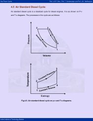
1.3 Analog versus digital signal processing
The signal processing operations involved in many applications like communication
systems, control systems, instrumentation, biomedical signal processing
etc can be implemented in two different ways
(1) Analog or continuous time method and
(2) Digital or discrete time method.
The analog approach to signal processing was dominant for many years. The
analog signal processing uses analog circuit elements such as resistors, capacitors,
transistors, diodes etc. With the advent of digital computer and
later microprocessor, the digital signal processing has become dominant now
adays.
The analog signal processing is based on natural ability of the analog system
to solve differential equations the describe a physical system. The solution
are obtained in real time. In contrast digital signal processing relies on numerical
calculations. The method may or may not give results in real time.
The digital approach has two main advantages over analog approach
(1) Flexibility: Same hardware can be used to do various kind of signal processing
operation,while in the core of analog signal processing one has to
design a system for each kind of operation.
(2) Repeatability: The same signal processing operation can be repeated
again and again giving same results, while in analog systems there may be
parameter variation due to change in temperature or supply voltage.
The choice between analog or digital signal processing depends on application.
One has to compare design time,size and cost of the implementation.
1.4 Classification of signals
As mentioned earlier, we will use the term signal to mean a real or complex
valued function of real variable(s). Let us denote the signal by x(t). The
variable t is called independent variable and the value x of t as dependent
variable. We say a signal is continuous time signal if the independent variable
t takesvaluesinaninterval.
For example tɛ(−∞, ∞),ortɛ[0, ∞] or t ɛ [T0,T1]
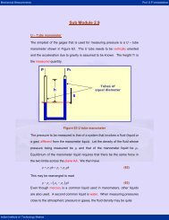
The independent variable t is referred to as time,even though it may not be
actually time. For example in variation if pressure with height t refers above
mean sea level.
When t takes a vales in a countable set the signal is called a discrete time
signal. For example
tɛ{0,T,2T,3T,4T, ...} or tɛ{... − 1, 0, 1, ...} or tɛ{1/2, 3/2, 5/2, 7/2, ...} etc.
2

For convenience of presentation we use the notation x[n] to denote discrete
time signal.
Let us pause here and clarify the notation a bit. When we write x(t) ithas
two meanings. One is value of x at time t and the other is the pairs(x(t),t)
allowable value of t. By signal we mean the second interpretation. To keep
this distinction we will use the following notation: {x(t)} to denote the continuous
time signal. Here {x(t)} is short notation for {x(t),tɛI} where I is
the set in which t takes the value. Similarly for discrete time signal we will
use the notation {x[n]}, where{x[n]} is short for {x[n],nɛI}. Note that in
{x(t)} and {x[n]} are dummy variables ie. {x[n]} and {x[t]} refer to the
same signal. Some books use the notation x[·] todenote{x[n]} and x[n] to
denote value of x at time n · x[n] refers to the whole waveform,while x[n]
refers to a particular value. Most of the books do not make this distinction
clean and use x[n] todenotesignalandx[n0] todenoteaparticularvalue.
As with independent variable t, the dependent variable x can take values in
a continues set or in a countable set. When both the dependent and independent
variable take value in intervals, the signal is called an analog signal.
When both the dependent and independent variables take values in countable
sets(two sets can be quite different) the signal is called Digital signal.When
we use digital computers to do processing we are doing digital signal processing.
But most of the theory is for discrete time signal processing where
default variable is continuous. This is because of the mathematical simplicity
of discrete time signal processing. Also digital signal processing tries to
implement this as closely as possible. Thus what we study is mostly discrete
time signal processing and what is really implemented is digital signal processing.
Exercise:
1.GIve examples of continues time signals.
2.Give examples of discrete time signals.
3.Give examples of signal where the independent variable is not time(onedimensional).
4.Given examples of signal where we have one independent variable but dependent
variable has more than one dimension.(This is sometimes called
vector valued signal or multichannel signal).
5.Give examples of signals where dependent variable is discrete but independent
variable are continues.
3

1.5 Elementary signals
There are several elementary signals that feature prominently in the study
of digital signals and digital signal processing.
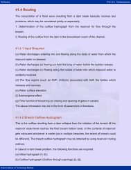
(a)Unit sample sequence δ[n]: Unit sample sequence is defined by
1, n =0
δ[n] =
0, n = 0
Graphically this is as shown below.
δ[n]
1
-3 -2 -1 0 1 2 3 4
Unit sample sequence is also known as impulse sequence. This plays role akin
to the impulse function δ(t) of continues time. The continues time impulse
δ(t) is purely a mathematical construct while in discrete time we can actually
generate the impulse sequence.
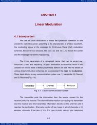
(b)Unit step sequence u[n]: Unit step sequence is defined by
1, n ≥ 0
u[n] =
0, n < 0
Graphically this is as shown below
u[n]
..........
1
-3 -2 -1 0 1 2 3 4
.................
................
(c) Exponential sequence: The complex exponential signal or sequence x[n]
is defined by
n
n
x[n] =Cα n
where C and α are, in general, complex numbers. Note that by writing
α = e β , we can write the exponential sequence as x[n] =ce βn .
4

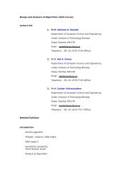
Real exponential signals: If C and α are real, we can have one of the several
type of behavior illustrated below
. . . . . . . . . .
. . . . . . . . . .
. . . . . . . . . .
. . . . . . . . . .
n
n
n
n
{x[n] =α n ,α>1}
{x[n] =α n , 0

Thus for |α| = 1, the real and imaginary parts of a cmplex exponential
sequence are sinusoidal. For |α| < 1, they correspond to sinusoidal sequence
multiplied by a decaying exponential, and for |α| > 1 they correspond to
sinusiodal sequence multiplied by a growing exponential.
1.6 Generating Signals with MATLAB
MATLAB, acronym for MATrix LABoratory has become a very porplar software
environment for complex based study of signals and systems. Here we
give some sample programmes to generate the elementary signals discussed
above. For details one should consider MATLAB manual or read help files.
In MATLAB, ones(M,N) is an M-by-N matrix of ones, and zeros(M,N) is an
M-by-N matrix of zeros. We may use those two matrices to generate impulse
and step sequence.
The following is a program to generate and display impulse sequence.
>> % Program to generate and display impulse response sequence
>> n = −49 : 49;
>> delta =[zeros(1, 49), 1,zeros(1, 49)];
>> stem(n, delta)
Here >> indicates the MATLAB prompt to type in a command, stem(n,x)
depicts the data contained in vector x as a discrete time signal at time values
defined by n. One can add title and lable the axes by suitable commands.
To generate step sequence we can use the following program
>> % Program to generate and display unit step function
>> n = −49 : 49;
>> u =[zeros(1, 49),ones(1, 50)];
>> stem(n, u);
We can use the following program to generate real exponential sequence
>> % Program to generate real exponential sequence
>> C =1;
>> alpha =0.8;
>> n = −10 : 10;
>> x = C ∗ alpha. ∧ n
>> stem(n, x)
Note that, in their program, the base alpha is a scalar but the exponent is a
vector, hence use of the operator .∧ to denote element-by-element power.
Exercise: Experiment with this program by changing different values of alpha
(real). Values of alpha greater then 1 will give growing exponential and
less than 1 will give decaying exponentials.
6