Statistical Mechanics - Physics at Oregon State University

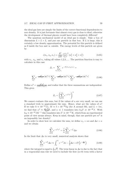
3.7. IDEAL GAS IN FIRST APPROXIMATION. 59
the ideal gas laws are simply the limits of the correct functional dependencies to
zero density. It is just fortunate that almost every gas is close to ideal, otherwise
the development of thermal physics would have been completely different!
The quantum mechanical model of an ideal gas is simple. Take a box of
dimensions L × L × L, and put one particle in that box. If L is large, this is
certainly a low density approximation. The potential for this particle is defined
as 0 inside the box and ∞ outside. The energy levels of this particle are given
by
ɛ(nx, ny, nz) = 2
π
2 (n
2M L
2 x + n 2 y + n 2 z) (3.85)
with nx ,ny, and nz taking all values 1,2,3,..... The partition function is easy to
calculate in this case
nx
2 − 2Mk e B T ( π
L) 2 n 2
x
Z1 =
ny
nxnynz
e −βɛ(nxnynz) =
2 − 2Mk e B T ( π
L) 2 n 2
y
nz
2 − 2Mk e B T ( π
L) 2 n 2
z (3.86)
Define α2 =
2 π 2
(2ML2kBT ) and realize that the three summations are independent.
This gives
∞
Z1 = e −α2n 2
n=1
3
(3.87)
We cannot evaluate this sum, but if the values of α are very small, we can use
a standard trick to approximate the sum. Hence, what are the values of α?
If we take ≈ 10 −34 Js, M ≈ 5 × 10 −26 kg (for A around 50), and L = 1m,
we find that α 2 ≈ 10−38 J
kBT , and α ≪ 1 translates into kBT ≫ 10 −38 J. With
kB ≈ 10 −23 JK −1 this translates into T ≫ 10 −15 K, which from an experimental
point of view means always. Keep in mind, though, that one particle per m 3 is
an impossibly low density!
In order to show how we calculate the sum, we define xn = αn and ∆x = α
and we obtain
∞
e −α2n 2
n=1
= 1
α
∞
n=1
e −x2n∆x
(3.88)
In the limit that ∆x is very small, numerical analysis shows that
∞
n=1
e −x2n∆x
≈
∞
e −x2
0
dx − 1
1 −
∆x + O e ∆x
2
(3.89)
where the integral is equal to 1√
2 π. The term linear in ∆x is due to the fact that
in a trapezoidal sum rule we need to include the first (n=0) term with a factor