Statistical Mechanics - Physics at Oregon State University

More documents

Recommendations

Info

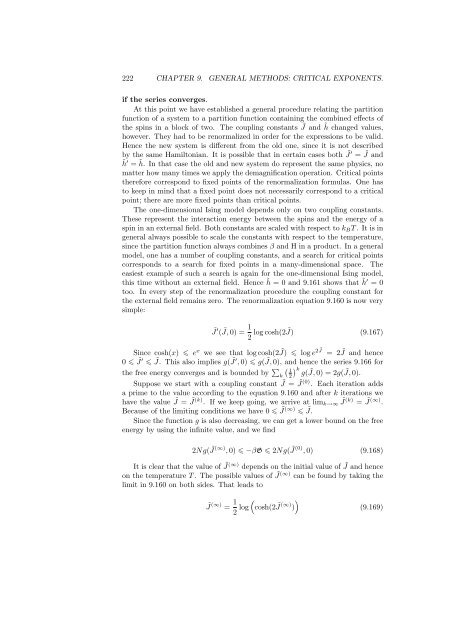
222 CHAPTER 9. GENERAL METHODS: CRITICAL EXPONENTS. if the series converges. At this point we have established a general procedure relating the partition function of a system to a partition function containing the combined effects of the spins in a block of two. The coupling constants ˜ J and ˜ h changed values, however. They had to be renormalized in order for the expressions to be valid. Hence the new system is different from the old one, since it is not described by the same Hamiltonian. It is possible that in certain cases both ˜ J ′ = ˜ J and ˜h ′ = ˜ h. In that case the old and new system do represent the same physics, no matter how many times we apply the demagnification operation. Critical points therefore correspond to fixed points of the renormalization formulas. One has to keep in mind that a fixed point does not necessarily correspond to a critical point; there are more fixed points than critical points. The one-dimensional Ising model depends only on two coupling constants. These represent the interaction energy between the spins and the energy of a spin in an external field. Both constants are scaled with respect to kBT . It is in general always possible to scale the constants with respect to the temperature, since the partition function always combines β and H in a product. In a general model, one has a number of coupling constants, and a search for critical points corresponds to a search for fixed points in a many-dimensional space. The easiest example of such a search is again for the one-dimensional Ising model, this time without an external field. Hence ˜ h = 0 and 9.161 shows that ˜ h ′ = 0 too. In every step of the renormalization procedure the coupling constant for the external field remains zero. The renormalization equation 9.160 is now very simple: ˜J ′ ( ˜ J, 0) = 1 2 log cosh(2 ˜ J) (9.167) Since cosh(x) ex we see that log cosh(2 ˜ J) log e2 ˜ J = 2J˜ and hence 0 ˜ J ′ ˜ J. This also implies g( ˜ J ′ , 0) g( ˜ J, 0), and hence the series 9.166 for the free energy converges and is bounded by 1 k k 2 g( J, ˜ 0) = 2g( J, ˜ 0). Suppose we start with a coupling constant ˜ J = ˜ J (0) . Each iteration adds a prime to the value according to the equation 9.160 and after k iterations we have the value ˜ J = ˜ J (k) . If we keep going, we arrive at limk→∞ ˜ J (k) = ˜ J (∞) . Because of the limiting conditions we have 0 ˜ J (∞) ˜ J. Since the function g is also decreasing, we can get a lower bound on the free energy by using the infinite value, and we find 2Ng( ˜ J (∞) , 0) −βG 2Ng( ˜ J (0) , 0) (9.168) It is clear that the value of ˜ J (∞) depends on the initial value of ˜ J and hence on the temperature T . The possible values of ˜ J (∞) can be found by taking the limit in 9.160 on both sides. That leads to ˜J (∞) = 1 2 log cosh(2 ˜ J (∞) ) (9.169)
9.7. RENORMALIZATION GROUP THEORY. 223 This equation has solutions ˜ J (∞) = 0 and ˜ J (∞) = ∞. These solutions are called the fixed points of the equation. If we start with one of these values, the scaling transformations will not change the values. Hence they represent physical situations that are length independent. In the case ˜ J (∞) = 0 we find that the free energy is given by −βG = 2N 1 4 log(4) = log(2N ) (9.170) The right hand side is equal to the entropy of a completely disordered chain divided by the Boltzmann constant. Therefore we have G = −T S, as expected for large temperatures or zero coupling constant. In the case ˜ J (∞) = ∞ we find that the free energy is given by −βG = 2N 1 4 log(2e2 ˜ J (∞) ) ⇒ G ≈ −NkBT ˜ J = −NJ (9.171) The right hand side is equal to the energy of a completely ordered chain, which happens if the temperature is zero of the coupling constant is infinity. If we start with an arbitrary value of ˜ J the next value will be smaller and so on. So we will end at the fixed point zero. The only exception is when we start exactly at infinity, then we stay at infinity. Hence we can say the following. If we start at a fixed point, we remain at that point. If we make a small deviation from the fixed point for our starting value, we always end up at zero. Therefore, ˜J (∞) = 0 is a stable fixed point and ˜ J (∞) = ∞ is an unstable fixed point. The stable fixed point ˜ J = 0 corresponds to T = ∞. At an infinite temperature any system is completely disordered and the states of the individual spins are completely random and uncorrelated. If we average random numbers the results will remain random and a system at an infinite temperature will look the same for any magnification. This fixed point is therefore a trivial fixed point and is expected to occur for any system. The same is true for the second fixed point in our simple model, which corresponds to T = 0. At zero temperature all spins are ordered and again the system looks the same under any magnification. It is again a fixed point which will always show up. It does not correspond to a critical point since it does not divide the temperature range in two parts, there are no negative temperatures. Close to zero temperature the effects of this fixed point are noticeable, however, and show up in a divergence of the correlation length to infinity at T = 0. Note that at infinite temperature the correlation length becomes zero. What we do in renormalization group theory is to replace one spin by the effective value of a block of spins. That changes the length scales of our problem, and in general changes our observations. That is not true, however, at the critical point. In that case the correlation length is infinity and repeated transformations will give the same results. Therefore , the critical point will show up as a fixed point in the scaling equations. The other case where changing length scales does not affect the physics is when the correlation length is zero. Hence we always have a fixed point corresponding to zero correlation length or infinite temperature.
Page 1:
Statistical Mechanics Henri J.F. Ja
Page 4 and 5:
IV CONTENTS 4.3 Gas of poly-atomic
Page 6 and 7:
VI CONTENTS
Page 8 and 9:
VIII INTRODUCTION Introduction. The
Page 10 and 11:
X INTRODUCTION In chapter nine we d
Page 12 and 13:
2 CHAPTER 1. FOUNDATION OF STATISTI
Page 14 and 15:
Page 16 and 17:
Page 18 and 19:
Page 20 and 21:
10 CHAPTER 1. FOUNDATION OF STATIST
Page 22 and 23:
Page 24 and 25:
Page 26 and 27:
Page 28 and 29:
Page 30 and 31:
Page 32 and 33:
Page 34 and 35:
24 CHAPTER 2. THE CANONICAL ENSEMBL
Page 36 and 37:
Page 38 and 39:
Page 40 and 41:
Page 42 and 43:
Page 44 and 45:
Page 46 and 47:
Page 48 and 49:
Page 50 and 51:
Page 52 and 53:
Page 54 and 55:
44 CHAPTER 3. VARIABLE NUMBER OF PA
Page 56 and 57:
Page 58 and 59:
Page 60 and 61:
Page 62 and 63:
Page 64 and 65:
Page 66 and 67:
Page 68 and 69:
Page 70 and 71:
Page 72 and 73:
Page 74 and 75:
Page 76 and 77:
Page 78 and 79:
68 CHAPTER 4. STATISTICS OF INDEPEN
Page 80 and 81:
Page 82 and 83:
Page 84 and 85:
Page 86 and 87:
Page 88 and 89:
Page 90 and 91:
Page 92 and 93:
Page 94 and 95:
Page 96 and 97:
Page 98 and 99:
Page 100 and 101:
90 CHAPTER 5. FERMIONS AND BOSONS
Page 102 and 103:
92 CHAPTER 5. FERMIONS AND BOSONS t
Page 104 and 105:
94 CHAPTER 5. FERMIONS AND BOSONS w
Page 106 and 107:
96 CHAPTER 5. FERMIONS AND BOSONS T
Page 108 and 109:
98 CHAPTER 5. FERMIONS AND BOSONS S
Page 110 and 111:
Page 112 and 113:
Page 114 and 115:
Page 116 and 117:
Page 118 and 119:
Page 120 and 121:
Page 122 and 123:
Page 124 and 125:
Page 126 and 127:
Page 128 and 129:
Page 130 and 131:
120 CHAPTER 6. DENSITY MATRIX FORMA
Page 132 and 133:
Page 134 and 135:
Page 136 and 137:
Page 138 and 139:
Page 140 and 141:
Page 142 and 143:
Page 144 and 145:
Page 146 and 147:
Page 148 and 149:
Page 150 and 151:
140 CHAPTER 7. CLASSICAL STATISTICA
Page 152 and 153:
Page 154 and 155:
Page 156 and 157:
Page 158 and 159:
Page 160 and 161:
Page 162 and 163:
Page 164 and 165:
Page 166 and 167:
Page 168 and 169:
158 CHAPTER 8. MEAN FIELD THEORY: C
Page 170 and 171:
Page 172 and 173:
Page 174 and 175:
Page 176 and 177:
Page 178 and 179:
Page 180 and 181:
Page 182 and 183: 172 CHAPTER 8. MEAN FIELD THEORY: C
Page 202 and 203: 192 CHAPTER 9. GENERAL METHODS: CRI
Page 240 and 241: 230 APPENDIX A. SOLUTIONS TO SELECT
Page 270: 260 APPENDIX A. SOLUTIONS TO SELECT
show all

Statistical Mechanics - Physics at Oregon State University

Create successful ePaper yourself

Delete template?

Save as template?