Statistical Mechanics - Physics at Oregon State University

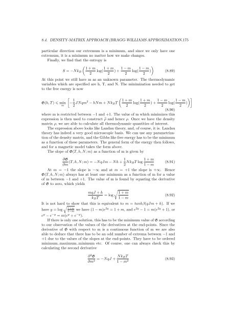
8.4. DENSITY-MATRIX APPROACH (BRAGG-WILLIAMS APPROXIMATION.175
particular direction our extremum is a minimum, and since we only have one
extremum, it is a minimum no matter how we make changes.
Finally, we find that the entropy is
1 + m 1 + m 1 − m 1 − m
S = −NkB log( ) + log( ) (8.89)
2 2 2 2
At this point we still have m as an unknown parameter. The thermodynamic
variables which are specified are h, T, and N. The minimization needed to get
to the free energy is now
G(h, T ) min
m
− 1
2 JNqm2
1 + m
− hNm + NkBT log(
2
1 + m 1 − m
) +
2 2
(8.90)
where m is restricted between −1 and +1. The value of m which minimizes this
expression is then used to construct ρ and hence ρ. Once we have the density
matrix ρ, we are able to calculate all thermodynamic quantities of interest.
The expression above looks like Landau theory, and, of course, it is. Landau
theory has indeed a very good microscopic basis. We can use any parametrization
of the density matrix, and the Gibbs like free energy has to be the minimum
as a function of these parameters. The general form of the energy then follows,
and for a magnetic model takes the form above.
The slope of G(T, h, N; m) as a function of m is given by
∂G
1
(T, h, N; m) = −NqJm − Nh +
∂m 2 NkBT
1 + m
log (8.91)
1 − m
At m = −1 the slope is −∞ and at m = +1 the slope is +∞. Hence
G(T, h, N; m) always has at least one minimum as a function of m for a value
of m between −1 and +1. The value of m is found by equating the derivative
of G to zero, which yields
mqJ + h 1 + m
= log
(8.92)
kBT 1 − m
It is not hard
to show that this is equivalent to m = tanhβ(qJm + h). If we
1+m
have y = log 1−m we have (1 − m)e2y = 1 + m, and e2y − 1 = m(e2y + 1), or
ey − e−y = m(ey + e−y ).
If there is only one solution, this has to be the minimum value of G according
to our observation of the values of the derivatives at the end-points. Since the
derivative of G with respect to m is a continuous function of m we are also
able to deduce that there has to be an odd number of extrema between −1 and
+1 due to the values of the slopes at the end-points. They have to be ordered
minimum..maximum..minimum etc. Of course, one can always check this by
calculating the second derivative
∂2G NkBT
= −NqJ +
∂m2 1 − m2 log(
(8.93)
1 − m
)
2