Statistical Mechanics - Physics at Oregon State University

5.1. FERMIONS IN A BOX. 101
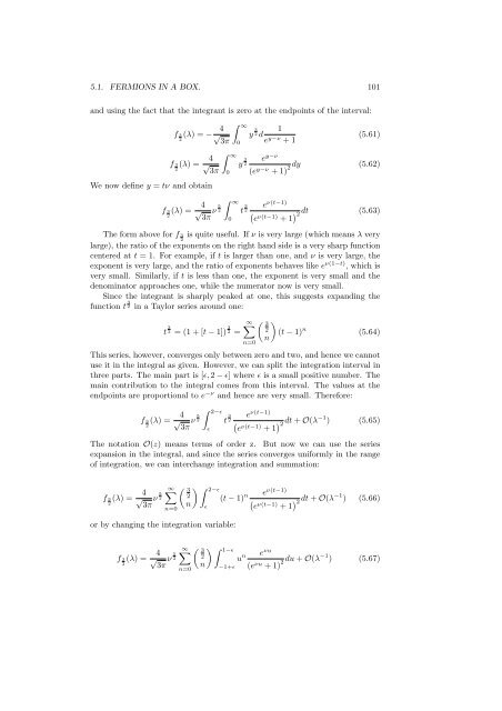
and using the fact that the integrant is zero at the endpoints of the interval:
∞
y 3 1
2 d
ey−ν (5.61)
+ 1
4
f 3 (λ) = −√ 2 3π
4
f 3 (λ) = √
2 3π
We now define y = tν and obtain
The form above for f 3
2
4
f 3 (λ) = √ ν
2 3π 5
2
∞
0
0
∞
0
y 3
2
t 3
2
ey−ν (ey−ν 2 dy (5.62)
+ 1)
e ν(t−1)
e ν(t−1) + 1 2 dt (5.63)
is quite useful. If ν is very large (which means λ very
large), the ratio of the exponents on the right hand side is a very sharp function
centered at t = 1. For example, if t is larger than one, and ν is very large, the
exponent is very large, and the ratio of exponents behaves like e ν(1−t) , which is
very small. Similarly, if t is less than one, the exponent is very small and the
denominator approaches one, while the numerator now is very small.
Since the integrant is sharply peaked at one, this suggests expanding the
function t 3
2 in a Taylor series around one:
t 3
2 = (1 + [t − 1]) 3
2 =
∞
n=0
3
2
n
(t − 1) n
(5.64)
This series, however, converges only between zero and two, and hence we cannot
use it in the integral as given. However, we can split the integration interval in
three parts. The main part is [ɛ, 2 − ɛ] where ɛ is a small positive number. The
main contribution to the integral comes from this interval. The values at the
endpoints are proportional to e −ν and hence are very small. Therefore:
4
f 3 (λ) = √ ν
2 3π 5
2
2−ɛ
ɛ
t 3
2
e ν(t−1)
e ν(t−1) + 1 2 dt + O(λ −1 ) (5.65)
The notation O(z) means terms of order z. But now we can use the series
expansion in the integral, and since the series converges uniformly in the range
of integration, we can interchange integration and summation:
4
f 3 (λ) = √ ν
2 3π 5
2
∞
3 2−ɛ
2 (t − 1)
n ɛ
n eν(t−1)
eν(t−1) 2 dt + O(λ
+ 1 −1 ) (5.66)
n=0
or by changing the integration variable:
4
f 3 (λ) = √ ν
2 3π 5
2
∞
n=0
3 1−ɛ
2
n −1+ɛ
u n eνu (eνu + 1) 2 du + O(λ−1 ) (5.67)