New Approaches to ElectroWeak Symmetry Breaking - LPSC
New Approaches to ElectroWeak Symmetry Breaking - LPSC
New Approaches to ElectroWeak Symmetry Breaking - LPSC

Create successful ePaper yourself
Turn your PDF publications into a flip-book with our unique Google optimized e-Paper software.
<strong>New</strong> <strong>Approaches</strong> <strong>to</strong><br />
<strong>ElectroWeak</strong> <strong>Symmetry</strong> <strong>Breaking</strong><br />
E = mc 2<br />
E = ¯hν<br />
Part Two<br />
Higgs as a (Pseudo) Gols<strong>to</strong>ne Boson: Little Higgs Theories.<br />
Higgs as a component of a Gauge Field: Gauge Higgs Unification.<br />
Ch!"ophe Grojean<br />
( chris<strong>to</strong>phe.grojean@cern.ch )<br />
Rµν − 1<br />
2 Rgµν = 16πG Tµν<br />
CERN-TH & Service de Physique Théorique - CEA Saclay
How <strong>to</strong> Stabilize the Higgs Potential<br />
Golds<strong>to</strong>ne’s Theorem<br />
spontaneously broken global symmetry massless scalar<br />
The spin trick<br />
a particle of spin s:<br />
... but the Higgs has sizable non-derivative<br />
couplings<br />
2s+1 polarization states<br />
...with the only exception of a particle moving at the<br />
speed of light<br />
... fewer polarization states<br />
Spin 1 Gauge invariance no longitudinal polarization<br />
Spin 1/2<br />
→<br />
→<br />
Chiral symmetry only one helicity<br />
→<br />
... but the Higgs is a spin 0 particle<br />
→<br />
m=0<br />
Ch!"ophe Grojean <strong>New</strong> approaches <strong>to</strong> <strong>ElectroWeak</strong> <strong>Symmetry</strong> <strong>Breaking</strong> 2 Lecture
Symmetries <strong>to</strong> Stabilize a Scalar Potential<br />
Supersymmetry<br />
Higher Dimensional<br />
Lorentz invariance<br />
fermion ~ boson<br />
Aµ ∼ A5<br />
4D spin 1 4D spin 0<br />
These symmetries cannot be exact symmetry of the Nature.<br />
They have <strong>to</strong> be broken. We want <strong>to</strong> look for a soft breaking in<br />
order <strong>to</strong> preserve the stabilization of the weak scale.<br />
Ch!"ophe Grojean <strong>New</strong> approaches <strong>to</strong> <strong>ElectroWeak</strong> <strong>Symmetry</strong> <strong>Breaking</strong> 2 Lecture
Li%le Higgs 'eo!es<br />
Ch!"ophe Grojean <strong>New</strong> approaches <strong>to</strong> <strong>ElectroWeak</strong> <strong>Symmetry</strong> <strong>Breaking</strong> 2 Lecture
U(1)<br />
φ = 1<br />
√ 2 (f + h(x)) e iθ(x)/f<br />
L = 1<br />
2∂µh∂ µ h + 1<br />
2<br />
Golds<strong>to</strong>ne Boson<br />
φ → e iα φ<br />
L = ∂µφ † ∂ µ φ − λ<br />
f+h<br />
f<br />
h → h<br />
θ → θ + αf<br />
2<br />
φ 2 2 −<br />
U(1)<br />
non-linearly realized<br />
shift symmetry forbids any mass term<br />
for θ<br />
Ch!"ophe Grojean <strong>New</strong> approaches <strong>to</strong> <strong>ElectroWeak</strong> <strong>Symmetry</strong> <strong>Breaking</strong> 2 Lecture<br />
f 2<br />
2<br />
2<br />
∂µθ∂ µ θ − λ f 2 h 2 + fh 3 + 1<br />
4 h4<br />
If the U(1) symmetry is gauged, the Golds<strong>to</strong>ne boson is<br />
eaten and it becomes the longitudinal component of<br />
the massive gauge boson
Example of Uneaten Golds<strong>to</strong>ne Bosons<br />
SU(N) → SU(N − 1)<br />
〈φ〉 =<br />
⎛<br />
⎜<br />
⎝<br />
0<br />
.<br />
0<br />
f<br />
⎞<br />
⎟<br />
⎠<br />
φ = exp<br />
⎛<br />
⎜<br />
⎝<br />
(N 2 − 1) − (N − 1) 2 − 1 = 2N − 1<br />
Let us assume that only SU(N-1) is gauged: then the Golds<strong>to</strong>ne are uneaten.<br />
SU(N − 1)<br />
SU(N)<br />
SU(N − 1)<br />
i<br />
f<br />
⎛<br />
⎜<br />
⎝<br />
−π0<br />
Golds<strong>to</strong>ne bosons<br />
φ = e (N-1) complex, , and 1 real, , scalars<br />
iπ φ0 π π0<br />
φ → UN−1φ = UN−1e iπ U †<br />
φ → exp<br />
π →<br />
<br />
i<br />
UN−1<br />
α †<br />
α<br />
1<br />
Ch!"ophe Grojean <strong>New</strong> approaches <strong>to</strong> <strong>ElectroWeak</strong> <strong>Symmetry</strong> <strong>Breaking</strong> 2 Lecture<br />
. ..<br />
π1<br />
−π0 πN−1<br />
π⋆ 1 . . . π⋆ N−1 (N − 1)π0<br />
π0 π<br />
<br />
exp<br />
π † π0<br />
N−1UN−1φ0 = e<br />
<br />
†<br />
U N−1 =<br />
1<br />
linear transformations<br />
<br />
i<br />
π †<br />
π<br />
<br />
φ0 ≈ exp<br />
.<br />
⎞⎞<br />
⎛<br />
⎟⎟<br />
⎜<br />
⎟⎟<br />
⎜<br />
⎟⎟<br />
⎜<br />
⎠⎠<br />
⎝<br />
†<br />
iUN−1πU<br />
N−1φ0<br />
π0<br />
π † U †<br />
N−1<br />
<br />
i<br />
non-linear transformations<br />
π † + α †<br />
UN−1π<br />
π0<br />
<br />
π + α<br />
0<br />
.<br />
0<br />
f<br />
<br />
⎞<br />
⎟<br />
⎠<br />
φ0
The Desired Properties of a Little Higgs<br />
Unbroken SU(2)xU(1) gauge symmetry<br />
At least 21/2 doublet as a Golds<strong>to</strong>ne boson<br />
Break the G/H shift symmetry that protects the Higgs potential in a way<br />
<strong>to</strong> allow a quartic coupling and a mass term, as well as Yukawa interactions<br />
<strong>to</strong> guarantee the absence of quadratic divergences at one loop<br />
Implement the idea of Higgs = (Pseudo)-Golds<strong>to</strong>ne boson<br />
Kaplan, Georgi ‘84<br />
Kaplan, Georgi, Dimopoulos ‘84<br />
Ch!"ophe Grojean <strong>New</strong> approaches <strong>to</strong> <strong>ElectroWeak</strong> <strong>Symmetry</strong> <strong>Breaking</strong> 2 Lecture
Collective <strong>Breaking</strong><br />
The global symmetry is explicitly broken but only “collectively” !<br />
the symmetry is broken when two or more couplings in the Lagrangian<br />
are non-vanishing.<br />
Setting any one of these couplings <strong>to</strong> zero res<strong>to</strong>res the symmetry<br />
and therefore the masslessness of the Little Higgs<br />
⎛<br />
φ1 with 〈φ1〉 = f ⎝ 0<br />
⎞<br />
0 ⎠<br />
1<br />
and φ2 with 〈φ2〉 = f<br />
[SU(3)/SU(2)] 2<br />
2x(8-3)=10 Golds<strong>to</strong>ne<br />
Let us now gauge SU(3)<br />
L = |Dµφ1| 2 + |Dµφ2| 2<br />
Dµφi = ∂µφi − igAµφi<br />
vev<br />
SU(3)V → SU(2)V<br />
the 5 Golds<strong>to</strong>ne are eaten<br />
φi → Uiφi<br />
Arkani-Hamed et al. ‘02<br />
φi → Uφi and Aµ → UAµU †<br />
Ch!"ophe Grojean <strong>New</strong> approaches <strong>to</strong> <strong>ElectroWeak</strong> <strong>Symmetry</strong> <strong>Breaking</strong> 2 Lecture<br />
⎛<br />
⎝ 0<br />
0<br />
1<br />
requires U1 = U2<br />
Break SU(3)1 − SU(3)2. Gauge SU(3)1 + SU(3)2.<br />
in presence of the gauge coupling, only 5 Golds<strong>to</strong>ne<br />
The 5 extra would-be Golds<strong>to</strong>ne boson acquire a mass through the gauge coupling<br />
⎞<br />
⎠
[SU(3)/SU(2)] 2<br />
2x(8-3)=10 Golds<strong>to</strong>ne<br />
Collective <strong>Breaking</strong><br />
φ1 with 〈φ1〉 = f<br />
Let us now gauge SU(3)<br />
L = |Dµφ1| 2 + |Dµφ2| 2<br />
Dµφi = ∂µφi − igAµφi<br />
vev<br />
SU(3)V → SU(2)V<br />
the 5 Golds<strong>to</strong>ne are eaten<br />
Ch!"ophe Grojean <strong>New</strong> approaches <strong>to</strong> <strong>ElectroWeak</strong> <strong>Symmetry</strong> <strong>Breaking</strong> 2 Lecture<br />
⎛<br />
⎝ 0<br />
0<br />
1<br />
⎞<br />
⎠ and φ2 with 〈φ2〉 = f<br />
φi → Uiφi<br />
φi → Uφi and Aµ → UAµU †<br />
⎛<br />
⎝ 0<br />
0<br />
1<br />
requires U1 = U2<br />
Break SU(3)1 − SU(3)2. Gauge SU(3)1 + SU(3)2.<br />
in presence of the gauge coupling, only 5 Golds<strong>to</strong>ne<br />
The 5 extra would-be Golds<strong>to</strong>ne boson acquire a mass through the gauge coupling.<br />
As soon as the coupling of either φ1 <strong>to</strong> Aμ or φ2 <strong>to</strong> Aμ is set <strong>to</strong> zero, enlarged global<br />
symmetry and 5 Golds<strong>to</strong>ne in the physical spectrum.<br />
If a diagram involves only one type of couplings,<br />
it cannot generate a mass term for the pseudo-Golds<strong>to</strong>ne bosons<br />
There is no quadratically divergent diagrams at one loop.<br />
⎞<br />
⎠
Λ 2<br />
Absence of Λ 2 divergent Diagrams<br />
SU(3)<br />
φ †<br />
i<br />
Log (Λ 2 )<br />
φ2<br />
φ †<br />
1<br />
φi<br />
φ †<br />
2<br />
φ1<br />
δL = g2 Λ 2<br />
δL = g4 f 2<br />
16π 2<br />
16π<br />
2 (φ†<br />
1 φ1 + φ †<br />
2 φ2) = g2 f 2 Λ 2<br />
8π 2<br />
independent of the Higgs field!<br />
Ch!"ophe Grojean <strong>New</strong> approaches <strong>to</strong> <strong>ElectroWeak</strong> <strong>Symmetry</strong> <strong>Breaking</strong> 2 Lecture<br />
<br />
<br />
φ †<br />
1 φ2<br />
<br />
<br />
log Λ2<br />
Simplest Higgs<br />
Kaplan-Schmaltz ‘03<br />
Q2 = g4f 2<br />
Λ2<br />
log<br />
4π2 Q2 h† h<br />
log-divergent one-loop suppressed<br />
Higgs mass
Cancelation Mechanism of Λ 2<br />
<br />
φ1 = exp i<br />
<br />
φ2 = exp −i<br />
M 2 = g 2 f 2<br />
⎛<br />
⎜<br />
⎝<br />
1<br />
h †<br />
h †<br />
1<br />
h<br />
h<br />
1 − v2<br />
f 2<br />
<br />
<br />
f<br />
<br />
≈ f<br />
<br />
≈ f<br />
ih/f<br />
1 − (h † h)/(2f 2 )<br />
W’ cancels the quadratic divergences generated by W<br />
Ch!"ophe Grojean <strong>New</strong> approaches <strong>to</strong> <strong>ElectroWeak</strong> <strong>Symmetry</strong> <strong>Breaking</strong> 2 Lecture<br />
f<br />
1 − v2<br />
f 2<br />
v 2<br />
f 2<br />
v 2<br />
f 2<br />
−ih/f<br />
1 − (h † h)/(2f 2 )<br />
4<br />
3<br />
− v2<br />
f 2<br />
− v2<br />
√ 3f 2<br />
− v2<br />
√ 3f 2<br />
trM 2 is independent of v 2 ⇔ no quadratic divergence<br />
v 2<br />
f 2<br />
<br />
<br />
⎞<br />
⎟<br />
⎠
q =<br />
tL<br />
φ1 ≈ f<br />
φ2 ≈ f<br />
How <strong>to</strong> Generate a Yukawa Coupling<br />
bL<br />
<br />
<br />
<br />
y y<br />
≡ 2 of SU(2)<br />
ih/f<br />
1 − (h † h)/(2f 2 )<br />
−ih/f<br />
1 − (h † h)/(2f 2 )<br />
Q =<br />
Ch!"ophe Grojean <strong>New</strong> approaches <strong>to</strong> <strong>ElectroWeak</strong> <strong>Symmetry</strong> <strong>Breaking</strong> 2 Lecture<br />
⎛<br />
⎝<br />
L = y √ φ<br />
2 †<br />
1QtR + y √ φ<br />
2 †<br />
<br />
<br />
x<br />
yf<br />
T− TL T+<br />
tL<br />
− y<br />
2f<br />
L = yf<br />
tL<br />
bL<br />
TL<br />
2 QTR<br />
⎞<br />
⎠ ≡ 3 of SU(3)<br />
<br />
1 − h† h<br />
2f 2<br />
<br />
with<br />
+<br />
TLT+ + yh † qT−<br />
TR<br />
T+ = 1<br />
√ 2 (TR + tR) T− = i<br />
√ 2 (TR − tR)<br />
m 2 t = y 2 v 2<br />
m 2 T = y2 f 2<br />
<br />
1 − v2<br />
f 2<br />
trM 2 is independent of v 2 ⇔ no quadratic divergence<br />
heavy <strong>to</strong>p cancels the quadratic divergences generated by <strong>to</strong>p
Collective <strong>Breaking</strong> in the Top Sec<strong>to</strong>r<br />
Without Yukawa<br />
L = y √ 2 φ †<br />
1 QtR + y √ 2 φ †<br />
2 QTR<br />
φi → Uiφi<br />
SU(3) 2<br />
Global <strong>Symmetry</strong><br />
When both Yukawa are turned on φi → Uφi and Q → UQ<br />
we need both Yukawa <strong>to</strong> align the two SU(3)<br />
more than one coupling is required <strong>to</strong> break enough global symmetry<br />
<strong>to</strong> let the Higgs acquire a potential<br />
φ1<br />
no quadratically divergent diagram at one-loop !<br />
tR<br />
Q<br />
φ1<br />
φ2<br />
Q<br />
TR<br />
φ2<br />
<br />
Ch!"ophe Grojean <strong>New</strong> approaches <strong>to</strong> <strong>ElectroWeak</strong> <strong>Symmetry</strong> <strong>Breaking</strong> 2 Lecture<br />
d 4 k<br />
1<br />
(kµγ µ ∝ log Λ2<br />
− m) 4<br />
log-divergent contribution only
1. Bot<strong>to</strong>m Yukawa:<br />
Exercises<br />
Check that the bot<strong>to</strong>m mass is generated by<br />
2. Hypercharge:<br />
y φ1φ2QbR<br />
Show that you can introduce the hypercharge by simply<br />
extending the gauge symmetry <strong>to</strong> SU(3)xU(1)X<br />
hint: first determine the X charge of the two scalar triplets.<br />
Ch!"ophe Grojean <strong>New</strong> approaches <strong>to</strong> <strong>ElectroWeak</strong> <strong>Symmetry</strong> <strong>Breaking</strong> 2 Lecture
EWSB in Little Higgs<br />
At tree-level, no Higgs potential<br />
(well, a quartic coupling can be generated by integrating out another heavy Golds<strong>to</strong>ne)<br />
A quartic and a mass term are generated at one-loop.<br />
As in susy, the <strong>to</strong>p loop will generate a log-divergent tachyonic mass term<br />
that will trigger EWSB.<br />
Radiatively induced EWSB<br />
(that’s the dynamics of the model that drives the symmetry breaking, it is not arbitrary like in the SM)<br />
What<br />
we want<br />
Might be<br />
difficult<br />
v 2 = −m2<br />
2λ<br />
φ †<br />
1 φ2 = f 2<br />
large quartic (larger than v/f) in order <strong>to</strong> get<br />
a physical Higgs mass of order v and not v 2 /f.<br />
small mass term (of order v and not f)<br />
<br />
1 − 2 h† h<br />
f 2 + 2(h† h) 2<br />
3f 4<br />
Would be better <strong>to</strong> generate a tree-level quartic<br />
Ch!"ophe Grojean <strong>New</strong> approaches <strong>to</strong> <strong>ElectroWeak</strong> <strong>Symmetry</strong> <strong>Breaking</strong> 2 Lecture<br />
<br />
v ∼ f
Little Higgs with Tree Level Quartic<br />
Global symmetry<br />
Gauge symmetry<br />
v ∼ f/4π<br />
f<br />
SU(3)<br />
Σ1<br />
Σ2<br />
SU(2)<br />
x<br />
U(1)<br />
Ch!"ophe Grojean <strong>New</strong> approaches <strong>to</strong> <strong>ElectroWeak</strong> <strong>Symmetry</strong> <strong>Breaking</strong> 2 Lecture<br />
Σ3<br />
Σ4<br />
<br />
SU(3)L × SU(3)R/SU(3)V<br />
4<br />
SU(3) × SU(2) × U(1) → SU(2)l × U(1)y<br />
30, 21/2, 10<br />
not protected by<br />
collective breaking<br />
two complex doublets<br />
1 complex triplet<br />
1 complex singlet<br />
32 GB<br />
8 eaten<br />
24 PGB<br />
Will generate a quartic coupling<br />
for the light PGB<br />
Minimal moose model<br />
Arkani-Hamed, Cohen, Katz, Nelson, Gregoire, Wacker ‘02
"<br />
"<br />
f<br />
v ∼ f/4π<br />
4πf<br />
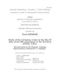
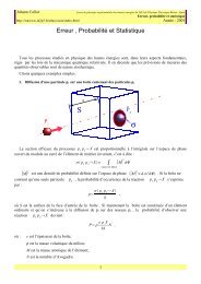
EW Precision Tests<br />
1 TeV<br />
100 GeV<br />
10 TeV<br />
!/2<br />
UV completion<br />
22 18<br />
4<br />
14 10 <strong>New</strong> particles (W’, Z’,<strong>to</strong>p’...)<br />
!/4<br />
!/4<br />
SM particles (Higgs,W,Z...)<br />
The new particles @ a TeV will affect 0 the EW precision 0 observables<br />
!/2<br />
!/4<br />
0<br />
!/2<br />
!/4<br />
22<br />
22<br />
SU(5) “littlest” Higgs model<br />
18<br />
18<br />
14<br />
14<br />
10<br />
0 !/4 !/2<br />
"'<br />
14<br />
10<br />
6<br />
SU(6) little Higgs model<br />
12<br />
10<br />
8<br />
6<br />
6<br />
"R<br />
!/2<br />
!/4<br />
8<br />
SO(9) little Higgs model<br />
6<br />
10<br />
4<br />
0<br />
0 !/4 !/2<br />
!/2<br />
"L<br />
8<br />
10<br />
6<br />
2<br />
4<br />
2<br />
3<br />
is computed at 99% C.L. for 1 dof, i.e. χ<br />
1<br />
Bounds from precision data on the scale f (in TeV)<br />
2<br />
for various Little Higgs models.<br />
2 = χ2 SM<br />
"<br />
!/4<br />
Incomplete SU(6) little Higgs model<br />
3<br />
4<br />
f>3-4 TeV 5 instead of f ~ 1 TeV<br />
6<br />
0 !/4<br />
"'<br />
!/2<br />
Ch!"ophe Grojean <strong>New</strong> approaches <strong>to</strong> <strong>ElectroWeak</strong> <strong>Symmetry</strong> <strong>Breaking</strong> 7<br />
2 Lecture<br />
"<br />
"<br />
!/2<br />
!/2<br />
!/4<br />
0<br />
22<br />
14<br />
SU(5) “littlest” Higgs model<br />
18<br />
14<br />
10<br />
6<br />
SU(6) little Higgs model<br />
12<br />
10<br />
8<br />
0 !/4 !/2<br />
"'<br />
6<br />
6<br />
"R<br />
"<br />
!/2<br />
!/4<br />
0<br />
8<br />
SO(9) little Higgs model<br />
6<br />
10<br />
0 !/4 !/2<br />
"L<br />
0 !/4 !/2<br />
2#<br />
8<br />
10<br />
Incomplete SU(6) little Higgs model<br />
Marandella, Schappacher, Strumia ‘05<br />
Figure 1: Bound from precision data on the scale f in TeV of little-Higgs models. The constraint<br />
+ 6.6. As described in the text in each model the<br />
angles φ parameterize the gauge couplings of the extra gauge groups, which become strongly coupled<br />
at φ → 0 and/or φ → π/2. The dotted iso-lines show that the constraint on f gets slightly relaxed<br />
in presence of arbitrary extra corrections <strong>to</strong> ˆ T . We assumed a light higgs, mh ∼ 115 GeV.<br />
3<br />
2<br />
6<br />
3<br />
4<br />
5<br />
6<br />
2<br />
1<br />
4<br />
2
Cus<strong>to</strong>dial <strong>Symmetry</strong> and T-parity<br />
To improve EW fits, two useful <strong>to</strong>ols:<br />
little Higgs with cus<strong>to</strong>dial symmetry<br />
T-parity<br />
Chang, Wacker ‘03 based on minimal moose with SO(5)...<br />
Cheng, Low ‘03<br />
heavy particles = odd<br />
light particles = even<br />
at each vertex, an even number of heavy fields are required<br />
no effective opera<strong>to</strong>r for light fields are generated<br />
by tree-level exchange of heavy fields<br />
tree-level exchange forbidden loop exchange allowed<br />
Ch!"ophe Grojean <strong>New</strong> approaches <strong>to</strong> <strong>ElectroWeak</strong> <strong>Symmetry</strong> <strong>Breaking</strong> 2 Lecture
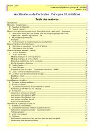
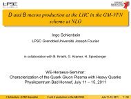
Fine-Tuning in Little Higgs<br />
!<br />
1000<br />
100<br />
10<br />
MSSM<br />
Littlest 2<br />
Littlest<br />
100 150 200 250 300 350 400<br />
m (GeV)<br />
h<br />
T-parity<br />
Simplest<br />
Figure 13: Comparative summary of the fine-tuning vs. mh for different scenarios. The curves for Little<br />
Casas, Espinosa, Hidalgo ‘05<br />
Higgs models (lines labeled “Littlest”, “Littlest 2”, “T -parity” and “Simplest”) are lower bounds on the<br />
corresponding fine-tuning, see text for details.<br />
corresponding <strong>to</strong> refs. [12, 13, 14, 15].<br />
Ch!"ophe Grojean <strong>New</strong> approaches <strong>to</strong> <strong>ElectroWeak</strong> <strong>Symmetry</strong> <strong>Breaking</strong> 2 Lecture<br />
SM
from the diagrams involving the BH. Certain choices of<br />
the fermion charges and the angle ψ ′ can help minimize<br />
these constraints [6]; alternately, the extra U(1) can be<br />
eliminated completely [9] without introducing significant<br />
fine tuning due <strong>to</strong> the smallness of the coupling g ′ . Given<br />
this model uncertainty in the U(1) sec<strong>to</strong>r, we will con-<br />
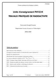
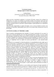
Experimental Signatures<br />
little Higgs models require a heavy <strong>to</strong>p and heavy gauge bosons<br />
centrate on the production and decay of the SU(2) heavy<br />
bosons.<br />
In pp collisions at the LHC, the heavy gauge bosons are<br />
predominantly produced through q¯q annihilation. The<br />
sub-process qg → WHq is considerably smaller and could<br />
be separately identified due <strong>to</strong> the presence of a high<br />
<strong>to</strong> guarantee the cancellation of the Λ2 divergences, the couplings<br />
of the new gauge bosons <strong>to</strong> the SM fermions is fixed<br />
pT jet. Fig. 3 shows the leading order production cross<br />
section of WH as a function of its mass, for the case<br />
ψ = π/4. The general case may be obtained from Fig.<br />
by simply scaling by cot2 ψ.<br />
Burdman, Perelstein, Pierce ‘02<br />
100 fb-1 (three years of LHC)<br />
FIG. 3. Production cross sections for W 3 H (solid) and W ±<br />
H<br />
(dashed) at the LHC, for ψ = π/4. We use the CTEQ5L<br />
par<strong>to</strong>n distribution function.<br />
production cross section<br />
of heavy W’ and Z’<br />
From our discussion thus far, it is clear that the twobody<br />
decay channels of the W 3 H include W 3 H → ¯ ff, where<br />
Partial width of ZH <strong>to</strong> fermions<br />
is proportional <strong>to</strong> cotan 2 θ<br />
Partial width of ZH in<strong>to</strong> boson pairs<br />
(Zh and W + W - )<br />
is proportional <strong>to</strong> cotan 2 2θ<br />
(this follows from the particuliar coupling of the<br />
Higgs <strong>to</strong> the two SU(2) gauge groups)<br />
cotan θ=g1/g2 (two SU(2) gauge couplings)<br />
Ch!"ophe Grojean <strong>New</strong> approaches <strong>to</strong> <strong>ElectroWeak</strong> <strong>Symmetry</strong> <strong>Breaking</strong> 2 Lecture
Gau)-Higgs Unification<br />
Ch!"ophe Grojean <strong>New</strong> approaches <strong>to</strong> <strong>ElectroWeak</strong> <strong>Symmetry</strong> <strong>Breaking</strong> 2 Lecture
Symmetries <strong>to</strong> Stabilize a Scalar Potential<br />
Higher Dimensional<br />
Lorentz invariance<br />
Aµ ∼ A5<br />
4D spin 1 4D spin 0<br />
These symmetries cannot be exact symmetry of the Nature.<br />
They have <strong>to</strong> be broken. We want <strong>to</strong> look for a soft breaking in<br />
order <strong>to</strong> preserve the stabilization of the weak scale.<br />
Ch!"ophe Grojean <strong>New</strong> approaches <strong>to</strong> <strong>ElectroWeak</strong> <strong>Symmetry</strong> <strong>Breaking</strong> 2 Lecture
How <strong>to</strong> Get a Doublet from an Adjoint<br />
Consider a 5D<br />
gauge symmetry G<br />
1<br />
2<br />
H ∼ A a 5<br />
will belong tho the adjoint rep. of G<br />
The SM Higgs is not an adjoint of SU(2)xU(1), it is a doublet !<br />
⎛<br />
⎜<br />
⎝<br />
SU(3)<br />
Consider a bigger gauge group<br />
G → SU(2)l × U(1)y<br />
Adj doublet + other rep.<br />
W3 + W8/ √ 3 W1 − iW2 W4 − iW5<br />
W1 + iW2 −W3 + W8/ √ 3 W6 − iW7<br />
W4 + iW5 W6 + iW7 −2W8/ √ 3<br />
Adj<br />
Ch!"ophe Grojean <strong>New</strong> approaches <strong>to</strong> <strong>ElectroWeak</strong> <strong>Symmetry</strong> <strong>Breaking</strong> 2 Lecture<br />
⎞<br />
⎟<br />
⎠<br />
SU(2)xU(1)<br />
2 √ 3/2
h+ = W4 − iW5<br />
h0 = W6 − iW7<br />
δT W = g 1<br />
2 √ 3<br />
⎛<br />
⎝<br />
U(1) Charge of the Doublet<br />
δT W = g [T, W ] T = 1<br />
2 √ 3<br />
1<br />
1<br />
−2<br />
= g 1<br />
2 √ 3<br />
⎞ ⎛<br />
⎠ ⎝<br />
⎛<br />
⎝<br />
−2h ⋆ +<br />
h ⋆ + h ⋆ 0<br />
−2h ⋆ 0<br />
= g 3<br />
2 √ 3<br />
h+<br />
h0<br />
⎛<br />
⎝<br />
⎛<br />
⎝ 1<br />
Ch!"ophe Grojean <strong>New</strong> approaches <strong>to</strong> <strong>ElectroWeak</strong> <strong>Symmetry</strong> <strong>Breaking</strong> 2 Lecture<br />
⎞<br />
⎠ − g 1<br />
2 √ 3<br />
h+<br />
h0<br />
⎞<br />
⎛<br />
⎝<br />
⎠ − g 1<br />
2 √ 3<br />
−h ⋆ + −h ⋆ 0<br />
h ⋆ + h ⋆ 0<br />
⎛<br />
⎝<br />
h+<br />
h ⋆ +<br />
h+<br />
U(1) charge of the doublet = 3<br />
2 √ 3<br />
h0<br />
⎞<br />
⎠<br />
h ⋆ 0<br />
h0<br />
1<br />
⎞ ⎛<br />
⎠ ⎝<br />
−2h+<br />
−2h0<br />
−2<br />
1<br />
⎞<br />
⎠<br />
⎞<br />
⎠<br />
1<br />
−2<br />
⎞<br />
⎠
Weak Mixing Angle<br />
δ U(1)<br />
h+<br />
h0<br />
<br />
= 3g<br />
2 √ 3<br />
h+<br />
Ch!"ophe Grojean <strong>New</strong> approaches <strong>to</strong> <strong>ElectroWeak</strong> <strong>Symmetry</strong> <strong>Breaking</strong> 2 Lecture<br />
h0<br />
<br />
=<br />
√ 3g<br />
2<br />
h+<br />
Proper U(1) normalization<br />
(such that the doublet has a hypercharge 1/2) g ′ = √ 3g U(1)y = T8/ √ 3<br />
sin 2 θW = g′2<br />
g2 3g2<br />
=<br />
+ g ′2 g2 3<br />
=<br />
+ 3g2 4<br />
By embedding SU(2)xU(1) in<strong>to</strong> a simple group, we got a<br />
prediction for the weak mixing angle<br />
experimentally: sin 2 θW ≈ 0.23<br />
h0<br />
<br />
Man<strong>to</strong>n ‘79<br />
Fairlie ‘79
How <strong>to</strong> Get a Good Weak Mixing Angle<br />
Repeat the previous construction with another gauge group<br />
G2 gauge group<br />
adjoint = 14 fundamental = 7<br />
SU(3) decomposition<br />
14 = 8 + 3 + ¯3 7 = 3 + ¯3 + 1<br />
T8 normalization<br />
14 =<br />
<br />
30 + (2 + ¯2) √ 3/2<br />
U(1)y normalization<br />
14 =<br />
<br />
+ 10<br />
30 + (2 + ¯2) 3/2 + 10<br />
<br />
+<br />
<br />
+<br />
SU(2)xU(1) decomposition<br />
<br />
2 + ¯2<br />
1/2 √ 3 +<br />
<br />
1 + ¯1<br />
−1/ √ 3<br />
<br />
2 + ¯2<br />
1/2 +<br />
U(1)y = √ 3 T8<br />
<br />
1 + ¯1<br />
−1<br />
Ch!"ophe Grojean <strong>New</strong> approaches <strong>to</strong> <strong>ElectroWeak</strong> <strong>Symmetry</strong> <strong>Breaking</strong> 2 Lecture<br />
7 =<br />
7 =<br />
Man<strong>to</strong>n ‘79<br />
Csáki, Grojean, Murayama ‘02<br />
<br />
2 + ¯2<br />
1/2 √ 3 +<br />
<br />
1 + ¯1<br />
−1/ √ 3<br />
<br />
2 + ¯2<br />
1/2 +<br />
<br />
1 + ¯1<br />
−1<br />
sin 2 θW = 1/4<br />
+ 10<br />
+ 10
fundamental rep.<br />
14 7x7 matrices<br />
T 9 = i<br />
2 √ 3<br />
λ 1 =<br />
⎛<br />
⎝<br />
λ 4 =<br />
⎛<br />
⎝<br />
0 1 0<br />
1 0 0<br />
0 0 0<br />
⎛<br />
⎝<br />
λ 7<br />
v 1†<br />
⎞<br />
0 0 1<br />
1 0 0<br />
0 0 0<br />
⎠ λ 2 =<br />
⎞<br />
v 1 =<br />
T a = 1<br />
2 √ 2<br />
v 1<br />
⎛<br />
⎝<br />
⎠ λ 5 =<br />
⎛<br />
⎞<br />
G2 Gymnastic<br />
0 −i 0<br />
i 0 0<br />
0 0 0<br />
⎛<br />
⎝<br />
⎝ −i√ 2<br />
0<br />
0<br />
⎛<br />
⎝<br />
0 0 −i<br />
0 0 0<br />
i 0 0<br />
⎞<br />
λ a<br />
⎠ T 10 = −i<br />
2 √ 3<br />
⎠ v 2 =<br />
−λ at<br />
⎛<br />
⎝<br />
with<br />
⎞ ⎛<br />
⎠ λ 3 =<br />
⎞<br />
Ch!"ophe Grojean <strong>New</strong> approaches <strong>to</strong> <strong>ElectroWeak</strong> <strong>Symmetry</strong> <strong>Breaking</strong> 2 Lecture<br />
⎝<br />
⎠ λ 6 =<br />
⎛<br />
⎝<br />
λ 5<br />
0<br />
i √ 2<br />
0<br />
⎞<br />
⎠ for a = 1 . . . 8<br />
v 2†<br />
1 0 0<br />
0 −1 0<br />
0 0 0<br />
⎛<br />
⎝<br />
⎞<br />
v 2<br />
⎠ v 3 =<br />
⎞<br />
⎠ T 11 = i<br />
2 √ 3<br />
T 12 = T 9† T 13 = T 10† T 14 = T 11† ,<br />
0 0 0<br />
0 0 1<br />
1 0 0<br />
⎛<br />
⎝<br />
⎞<br />
⎠ λ 8 = 1<br />
√ 3<br />
⎞<br />
⎠ λ 7 =<br />
0<br />
0<br />
−i √ 2<br />
Csáki, Grojean, Murayama ‘02<br />
⎞<br />
⎠ .<br />
⎛<br />
⎝<br />
⎛<br />
⎝<br />
⎛<br />
⎝<br />
λ 2<br />
v 3†<br />
1 0 0<br />
0 1 0<br />
0 0 −2<br />
0 0 0<br />
0 0 −i<br />
0 i 0<br />
⎞<br />
⎠<br />
v 3<br />
⎞<br />
⎠<br />
⎞<br />
⎠
6D for a Tree-level Quartic Coupling<br />
L = − 1<br />
4 F 2 µν + 1<br />
2 F 2 µ5 + 1<br />
2 F 2 µ6 − 1<br />
2 F 2 56<br />
F56 = ∂5A6 − ∂6A5 − g[A5, A6]<br />
A5 = H + . . . A6 = H + . . .<br />
L = −g 2 H 4<br />
An<strong>to</strong>niadis, Benakli, Quiros ‘01<br />
the 6D gauge kinetic term contains a Higgs quartic coupling<br />
and<br />
λ ≡ g 2<br />
Ch!"ophe Grojean <strong>New</strong> approaches <strong>to</strong> <strong>ElectroWeak</strong> <strong>Symmetry</strong> <strong>Breaking</strong> 2 Lecture
SU(3) model<br />
A5 =<br />
Explicit Tree-level Quartic<br />
⎛<br />
⎜<br />
⎝<br />
1<br />
2 h⋆ +<br />
Aµ = 1<br />
2<br />
⎛<br />
⎜<br />
⎝<br />
1<br />
2 h⋆ 0<br />
1<br />
2 h+<br />
1<br />
2 h0<br />
A 3 µ + 1<br />
3 A8 µ<br />
A 1 µ + iA 2 µ<br />
⎞<br />
Ch!"ophe Grojean <strong>New</strong> approaches <strong>to</strong> <strong>ElectroWeak</strong> <strong>Symmetry</strong> <strong>Breaking</strong> 2 Lecture<br />
⎛<br />
⎟<br />
⎠ A6<br />
⎜<br />
= ⎜<br />
⎝<br />
A 1 µ − iA 2 µ<br />
−A 3 µ + 1<br />
3 A8 µ<br />
i<br />
2 h⋆ +<br />
i<br />
2 h⋆ 0<br />
− 2<br />
√ 3 A 8 µ<br />
−i<br />
2 h+<br />
−i<br />
2 h0<br />
L = − 1<br />
2 Tr F 2 µν + Tr F 2 µ5 + Tr F 2 µ6 − Tr F 2 56<br />
L = DµH † DµH − g2<br />
2 (H† H) 2<br />
⎞<br />
⎟<br />
⎠<br />
⎞<br />
⎟<br />
⎠<br />
after orbifold<br />
projection...
πR<br />
−πR<br />
Towards a Complete Construction<br />
so far we haven’t broken any symmetry... we even enlarged the gauge group<br />
y<br />
−y<br />
We need <strong>to</strong> break G down <strong>to</strong> SU(2)xU(1)<br />
we can achieve this breaking while compactifying the extra-dimension<br />
0<br />
Orbifold Compactification <strong>Breaking</strong><br />
circle y ∼ y + 2πR<br />
⤶<br />
Z2 orbifold y ∼ −y<br />
U 2 = 1<br />
Aµ(−y) = UAµ(y)U † A5(−y) = −UA5(y)U †<br />
zero mode: is independent of<br />
Aµ<br />
Aµ = UAµU †<br />
Ch!"ophe Grojean <strong>New</strong> approaches <strong>to</strong> <strong>ElectroWeak</strong> <strong>Symmetry</strong> <strong>Breaking</strong> 2 Lecture<br />
y<br />
A5 = −UA5U †<br />
- signs are compensating<br />
gauge symmetry breaking + chiral fermions
Orbifold Projection as Boundary Conditions<br />
H subgroup<br />
A H µ (−y) = A H µ (y)<br />
A H 5 (−y) = −A H 5 (y)<br />
G/H coset<br />
A G/H<br />
µ<br />
A G/H<br />
5<br />
−πR<br />
(−y) = −A G/H<br />
µ<br />
(−y) = A G/H<br />
5<br />
y<br />
−y<br />
G → H by orbifold projection<br />
(y)<br />
(y)<br />
⤶Z2<br />
which is equivalent <strong>to</strong> the BCs<br />
at the fixed points<br />
which is equivalent <strong>to</strong> the BCs<br />
at the fixed points<br />
∂5A H µ = 0<br />
A H 5 = 0<br />
A G/H<br />
µ<br />
∂5A G/H<br />
5<br />
πR<br />
0<br />
U 2 ≈<br />
= 1 BC BC<br />
Ch!"ophe Grojean <strong>New</strong> approaches <strong>to</strong> <strong>ElectroWeak</strong> <strong>Symmetry</strong> <strong>Breaking</strong> 2 Lecture<br />
= 0<br />
= 0
SU(3) → SU(2)xU(1) 5D Orbifold <strong>Breaking</strong><br />
massless Aµ<br />
[Aµ, U] = 0 Aµ = 1<br />
2<br />
massless A5<br />
U =<br />
⎛<br />
⎝ −1<br />
⎛<br />
⎜<br />
⎝<br />
{A5, U} = 0 A5 = 1<br />
2<br />
A 3 µ + A 8 / √ 3 A 1 µ − iA 2 µ<br />
⎛<br />
⎜<br />
⎝<br />
−1<br />
A 1 µ + iA 2 µ<br />
1<br />
A 4 5 + iA 5 5<br />
−A 3 µ + A 8 µ/ √ 3<br />
A 6 5 + iA 7 5<br />
A 4 5 − iA 5 5<br />
A 6 5 − iA 7 5<br />
−2A 8 µ/ √ 3<br />
Ch!"ophe Grojean <strong>New</strong> approaches <strong>to</strong> <strong>ElectroWeak</strong> <strong>Symmetry</strong> <strong>Breaking</strong> 2 Lecture<br />
⎞<br />
⎠ U ∈ SU(3) U 2 = 1<br />
⎞<br />
⎟<br />
⎠<br />
⎞<br />
⎟<br />
⎠<br />
SU(2) × U(1)<br />
SU(3)<br />
SU(2) × U(1)
!<br />
2 R<br />
0<br />
U =<br />
⎛<br />
⎝ i<br />
z<br />
i<br />
0<br />
U 4 = 1<br />
T O<br />
−1<br />
⎞<br />
⎠<br />
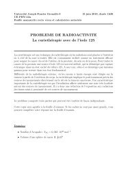
6D Orbifold <strong>Breaking</strong><br />
!<br />
2 R<br />
Ay =<br />
⎛<br />
⎜<br />
⎝<br />
Fundamental domain<br />
of the <strong>to</strong>rus<br />
Fundamental domain<br />
y<br />
1<br />
2 h⋆ +<br />
of the orbifold<br />
Fixed points<br />
of the orbifold<br />
T 2 /Z 4 orbifold<br />
y<br />
z<br />
Ch!"ophe Grojean <strong>New</strong> approaches <strong>to</strong> <strong>ElectroWeak</strong> <strong>Symmetry</strong> <strong>Breaking</strong> 2 Lecture<br />
1<br />
2 h⋆ 0<br />
1<br />
2 h+<br />
1<br />
2 h0<br />
⎞<br />
<br />
∼<br />
−z<br />
y<br />
<br />
Aµ(−z, y) = UAµ(y, z)U †<br />
Ay(−z, y) = −UAz(y, z)U †<br />
Az(−z, y) = UAy(y, z)U †<br />
⎛<br />
⎟<br />
⎠ Az<br />
⎜<br />
= ⎜<br />
⎝<br />
i<br />
2 h⋆ +<br />
i<br />
2 h⋆ 0<br />
−i<br />
2 h+<br />
−i<br />
2 h0<br />
⎞<br />
⎟<br />
⎠
In the bulk<br />
Residual <strong>Symmetry</strong><br />
higher dimensional gauge invariance forbids a mass term for A5<br />
At the fixed points<br />
G → H<br />
δA A M = ∂M ɛ A + gf ABC A B µ ɛ C<br />
⎧<br />
⎨<br />
⎩<br />
∂5A H µ = 0 A H 5 = 0 ∂5ɛ H = 0<br />
A G/H<br />
µ = 0 ∂5A G/H<br />
5 = 0 ɛ G/H = 0<br />
(since [H, H] ⊂ H [H, G/H] ⊂ G/H,<br />
the only non-vanishing structure constants are f HHH , f G/H G/H H )<br />
δA H µ = ∂µɛ H + gf HHH A H µ ɛ H<br />
δA H 5 = 0<br />
δA G/H<br />
µ<br />
δA G/H<br />
5<br />
= 0<br />
= ∂5ɛ G/H + gf G/H G/H H A G/H<br />
5<br />
G/H acts non-linearly on the Higgs at the fixed points.<br />
No local mass term allowed<br />
Ch!"ophe Grojean <strong>New</strong> approaches <strong>to</strong> <strong>ElectroWeak</strong> <strong>Symmetry</strong> <strong>Breaking</strong> 2 Lecture<br />
ɛ H<br />
Gersdorff, Irges, Quiros ‘02
Finite Mass from Wilson Line<br />
there is no local counter term that will give a mass <strong>to</strong> the Higgs<br />
the mass term can only be generated non locally<br />
the mass term will be finite then<br />
Wn = e i R 2nπR<br />
0 A5dy Wilson’s line. Gauge invariant object.<br />
The radiative corrections will generate a (finite) effective potential<br />
Veff (A5) = f(Wn)<br />
controlled by finite size effects<br />
UV insensitive<br />
Ch!"ophe Grojean <strong>New</strong> approaches <strong>to</strong> <strong>ElectroWeak</strong> <strong>Symmetry</strong> <strong>Breaking</strong> 2 Lecture
Tadpole Opera<strong>to</strong>r<br />
the situation complicates in 6D<br />
F56 contains a mass term for the Higgs<br />
Tr (U F56) is a local invariant opera<strong>to</strong>r at a fixed point<br />
Tr (UF56(0)) → Tr (Ug(0)F56(0)g −1 (0)) = Tr (UF56(0)g −1 (0)g(0)) = Tr (UF56(0))<br />
gauge loop<br />
at the fixed points, U and g commute<br />
Unless forbidden by a discrete symmetry,<br />
we expect this opera<strong>to</strong>r <strong>to</strong> be generated at one loop<br />
ghost loop<br />
Csáki, Grojean, Murayama ‘02<br />
Gersdorff, Irges, Quiros ‘02<br />
For Z2 or Z2 x Z2 orbifolds can define a parity<br />
that forbids the tadpole<br />
For Z4 orbifold, no such symmetry<br />
a Λ 2 tadpole is generated at one loop<br />
Ch!"ophe Grojean <strong>New</strong> approaches <strong>to</strong> <strong>ElectroWeak</strong> <strong>Symmetry</strong> <strong>Breaking</strong> 2 Lecture
Direct coupling:<br />
Non local couplings:<br />
Fermion Masses<br />
4D chiral matter U(1)y fractional charges<br />
Higgs Coupling<br />
<br />
localize fermions at the fixed points<br />
Λ 2 divergences<br />
forbidden by G/H shift symmetry<br />
W = Pe i R Aidx i<br />
Extra Massive Fermion in the Bulk<br />
d 5 x ¯ ψ(i¯σ µ ∂µ − m)ψ + δ(y1)ψχ + δ(y2)ψξ <br />
integrating out<br />
massive fermion<br />
<br />
d 4 x e −m|y1−y2|)<br />
ξ(y2)e i R Aidx i<br />
χ(y1)<br />
Froggatt-Nielsen<br />
mass suppression<br />
Ch!"ophe Grojean <strong>New</strong> approaches <strong>to</strong> <strong>ElectroWeak</strong> <strong>Symmetry</strong> <strong>Breaking</strong> 2 Lecture
Experimental Signatures<br />
the collider signals haven’t been studied in details<br />
(lack of fully realistic models?)<br />
the main predictions of these models are<br />
KK excitations of W,Z around 500 GeV ~ 1 TeV<br />
KK excitations of G/H: gauge bosons with the quantum numbers of the Higgs doublets<br />
extra scalar fields<br />
extra fermions (<strong>to</strong> cancel the <strong>to</strong>p loop quadratic divergence)<br />
Ch!"ophe Grojean <strong>New</strong> approaches <strong>to</strong> <strong>ElectroWeak</strong> <strong>Symmetry</strong> <strong>Breaking</strong> 2 Lecture
In 6D models<br />
enlarge the gauge group?<br />
Open Issues<br />
start with SU(3) and add kinetic terms at the fixed points <strong>to</strong> change the<br />
prediction of the weak mixing angle?<br />
In 5D models<br />
add large boundary kinetic terms<br />
add appropriate matter fields in the bulk<br />
warped space<br />
generate a large Higgs quartic<br />
good prediction for the weak mixing angle<br />
generate a large Higgs quartic coupling at one-loop<br />
Seems <strong>to</strong> be a promising way <strong>to</strong> proceed.<br />
Weakly coupled dual of composite Higgs models<br />
See Agashe, Contino, Pomarol ‘04-’05<br />
Ch!"ophe Grojean <strong>New</strong> approaches <strong>to</strong> <strong>ElectroWeak</strong> <strong>Symmetry</strong> <strong>Breaking</strong> 2 Lecture