STUDIES OF ENERGY RECOVERY LINACS AT ... - CASA
STUDIES OF ENERGY RECOVERY LINACS AT ... - CASA STUDIES OF ENERGY RECOVERY LINACS AT ... - CASA
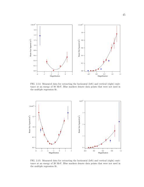
FIG. 2.14: Measured data for extracting the horizontal (left) and vertical (right) emittance at an energy of 56 MeV. Blue markers denote data points that were not used in the multiple regression fit. FIG. 2.15: Measured data for extracting the horizontal (left) and vertical (right) emittance at an energy of 20 MeV. Blue markers denote data points that were not used in the multiple regression fit. 45
ting the data is difficult. Without the ability to extract beam sizes in real time, this was only revealed after the fact. As with the previous measurement, fitting the complete data set results in an unphysical emittance. Since a unique beam size is expected for each value of the quadrupole strength, points were omitted that violated this condition. The result is a physically acceptable emittance. Horizontal Emittance: Einj = 20 MeV This data set represents an ideal measurement - a large number of data points with the beta function sweeping through a minimum. The two points that were omitted were outliers. Vertical Emittance: Einj = 20 MeV This measurement shows once again that the quadrupole strength was not suf- ficiently scanned and the fitting must be applied to half of a parabola. The points omitted were done so for obvious reasons; the rightmost point was omitted due to an excessively noisy wire scan (note the large error bar), while the other omitted point is an outlier. When scanning the quadrupole, not only is the energy recovered beam affected, but perhaps more importantly, so is the accelerated or first pass beam. The impor- tance results from the implicit assumption that the Twiss parameters at the entrance of the scanning quadrupole remain the same. In order to meet that requirement, a family of quadrupoles (downstream of the reinjection chicane) was used to produce compensating optics to counter the effects produced by the scanning quadrupole. Prior to the CEBAF-ER experiment, the emittance measurements were simu- lated in Optim [41], including producing appropriate compensatory optics. During the CEBAF-ER experiment however, the machine optics used for the Einj = 20 MeV configuration were not those used in the simulations. Hence, compensating op- 46
- Page 13 and 14: 2.10 Illustration of quadrupole sca
- Page 15 and 16: 5.1 Successive frames in time (prog
- Page 17 and 18: 6.8 A plot of 1/Qeff versus average
- Page 19 and 20: ABSTRACT An energy recovering linac
- Page 21 and 22: CHAPTER 1 Introduction An increasin
- Page 23 and 24: FIG. 1.1: Schematic of a generic li
- Page 25 and 26: FIG. 1.2: A CEBAF 5-cell cavity wit
- Page 27 and 28: The solution to Eq. (1.3) is U(t) =
- Page 29 and 30: y reducing the impedance of HOMs, a
- Page 31 and 32: Despite its success, this method of
- Page 33 and 34: design parameters, most notably ach
- Page 35 and 36: 1.4.2 Machine Optics The second cat
- Page 37 and 38: analytic model elucidates many impo
- Page 39 and 40: CHAPTER 2 CEBAF with Energy Recover
- Page 41 and 42: FIG. 2.1: Energy versus average cur
- Page 43 and 44: FIG. 2.3: Additional hardware insta
- Page 45 and 46: FIG. 2.4: A picture of the energy r
- Page 47 and 48: dipoles and beam diagnostics such a
- Page 49 and 50: FIG. 2.7: Horizontal (red) and vert
- Page 51 and 52: FIG. 2.8: Illustration of the cryom
- Page 53 and 54: linac and θNL is the RF phase. The
- Page 55 and 56: 2.4 Transverse Emittance One of the
- Page 57 and 58: where σ2 is the rms beam size meas
- Page 59 and 60: eams. The effects of varying the qu
- Page 61 and 62: FIG. 2.12: A typical wire scan near
- Page 63: quadratic fit and a multiple regres
- Page 67 and 68: primary source of error is measurin
- Page 69 and 70: identified, although the phase dela
- Page 71 and 72: TABLE 2.3: Comparison of Twiss para
- Page 73 and 74: the results of the fits. The vertic
- Page 75 and 76: FIG. 2.18: Schematic illustrating t
- Page 77 and 78: FIG. 2.19: The GASK signal measured
- Page 79 and 80: FIG. 2.20: The measured normalized
- Page 81 and 82: CHAPTER 3 The Jefferson Laboratory
- Page 83 and 84: FIG. 3.1: Schematic of the 10 kW FE
- Page 85 and 86: FIG. 3.2: Layout of the DC photocat
- Page 87 and 88: accelerating gradient at the front
- Page 89 and 90: eason for making the endloops achro
- Page 91 and 92: FIG. 3.7: Illustration of path leng
- Page 93 and 94: 3.5 Longitudinal Dynamics This sect
- Page 95 and 96: FIG. 3.9: The effect of a thin focu
- Page 97 and 98: Under the constraint that each orde
- Page 99 and 100: form of beam breakup not only occur
- Page 101 and 102: 4.1 The Pillbox Cavity Although the
- Page 103 and 104: FIG. 4.2: Electric field (red) and
- Page 105 and 106: where the full 4×4 transfer matrix
- Page 107 and 108: The threshold is inversely proporti
- Page 109 and 110: 4.3 BBU Simulation Codes: Particle
- Page 111 and 112: 6. The second pass beam bunch then
- Page 113 and 114: which excites it. The BBU instabili
FIG. 2.14: Measured data for extracting the horizontal (left) and vertical (right) emittance<br />
at an energy of 56 MeV. Blue markers denote data points that were not used in<br />
the multiple regression fit.<br />
FIG. 2.15: Measured data for extracting the horizontal (left) and vertical (right) emittance<br />
at an energy of 20 MeV. Blue markers denote data points that were not used in<br />
the multiple regression fit.<br />
45


