Codes over Gaussian integer rings - Telfor 2010

18th Telecommunications forum TELFOR 2010 Serbia, Belgrade, November 23-25, 2010.
Codes over Gaussian integer rings
Farhad Ghaboussi
Department of Computer Science
University of Applied Sciences Constance
Email: farhad.ghaboussi@htwg-konstanz.de
Web: www.edc.in.htwg-konstanz.de
Abstract—This work presents block codes over Gaussian
integer rings. Rings of Gaussian integers extend the number
of possible QAM signal constellations over Gaussian integer
fields. Many well-known code constructions can be used for
codes over Gaussian integer rings, e.g., the Plotkin construction
or product codes. These codes enable low complexity soft
decoding in the complex domain.
Index Terms—Gaussian integers, Plotkin construction,
product codes, soft input decoding
I. INTRODUCTION
Gaussian integers are a subset of the complex numbers
such that the real and imaginary parts are integers. Block
codes over Gaussian integers were first studied by Huber
in [1]. Huber also introduced the Mannheim distance as
a performance measure for codes over Gaussian integers.
Codes over Gaussian integers can be used for coding over
two-dimensional signal spaces, e.g. using QAM signals.
Similar code constructions were later considered in [2].
More recently, Gaussian integers were applied to construct
space-time codes [3], [4].
Most of the mentioned code constructions are linear
codes based on finite Gaussian integer fields which are
constructed from primes p of the form p ≡ 1mod4.The
number of signal points in these complex QAM constellations
is therefore limited to prime numbers satisfying
this condition, e.g. p = 5, 13, 17, 29,.... Additionally,
multiplicative groups were considered in [5].
In this work we consider code constructions over Gaussian
integer rings. Such rings can be used to construct
codes which are very similar to linear codes over Gaussian
integer fields. Gaussian integer rings can be constructed for
perfect squares. They have interesting algebraic properties.
We show that simple codes can be constructed similar
to the one Mannheim error correcting (OMEC) codes
presented by Huber in [1], by building product codes
as suggested by Elias [6] or using the so-called Plotkin
construction [7]. The recursive Plotkin construction can
also be exploited for low-complexity decoding [8], [10].
Similarly, the OMEC and product codes can be decoded
using Chase-type algorithms [11].
II. PRELIMINARIES
Gaussian integers are complex numbers such that the
real and imaginary parts are integers. The modulo function
μ(z) of a complex number z is defined as
∗ zπ
μ(z) =z mod π = z −
π · π∗
· π, (1)
Jürgen Freudenberger
Department of Computer Science
University of Applied Sciences Constance, Germany
Email: jfreuden@htwg-konstanz.de
Web: www.edc.in.htwg-konstanz.de
662
where π ∗ is the conjugate of the complex number π. [·]
denotes rounding to the closest Gaussian integer. That is,
for a complex number z = a+ib, wehave[z] =[a]+i [b].
We use the Mannheim weight and Mannheim distance as
introduced in [1]. Let the Mannheim weight of the complex
number z ∈Gm be defined as
wtM(z) =|Re {z}|+ |Im {z}|, (2)
then the Mannheim distance between two complex numbers
y and z is defined as
dM(y, z) =wtM(μ(z − y)) . (3)
Similarly, the Mannheim weight of the vector z is
wtM(z) =
wtM(μ(zi)) (4)
and the Mannheim distance for vectors is defined as
i
dM(y, z) =wtM(μ(z − y)) . (5)
The Mannheim distance defines a metric.
III. RINGS OF GAUSSIAN INTEGERS
Most of the code constructions in [1]–[4] are linear
codes based on finite Gaussian integer fields which are
constructed from primes p of the form p ≡ 1mod4.For
prime numbers p = 4c +1,c ∈ N the Gaussian field
structure is shown in [12].
We show in the following that the residue class ring
of Gaussian integers arises from the residue class ring of
certain integers with a unique quadratic decomposition.
Theorem 1: Given any non-prime integer m ∈ N with a
unique decomposition
m = a 2 + b 2 =(a + ib)(a − ib) =Π· Π ∗ ; a, b ∈ Z
there exists the residue class ring of Gaussian integers
modulo Π
Gm = {0,z c 1 ,zc 2 ,...,zc m−1 }
with elements
z c j := zj − [ zj · Π∗ ] · Π (6)
Π · Π∗ where [·] denotes rounding to the next Gaussian integer.
Proof: Zm = {0, 1,...,m− 1} is a residue class
ring [9]. Equation (6) is an isomorphic map, because there
exist an inverse map
zj =(z c j · s · Π∗ + z c∗
j · t · Π) mod m, (7)
where 1=s · Π ∗ + t · Π. s and t can be calculated using
the Euclidean algorithm [1].

Then for all z1,z2 ∈ Zm and all z c 1,z c 2 ∈Gm we have
the following ring homomorphism
according to
mod Π
z1 + z2 mod m ↔ z c 1 + zc 2
z1 · z2 mod m ↔ z c 1 · z c 2 mod Π
z c 1 + z c 2 mod Π = z c 1 + z c 2 − [ (z1 + z2) · Π ∗
Π · Π ∗
z c 1 · z c 2 mod Π = z c 1 · z c 2 − [ (z1 · z2) · Π ∗
Π · Π ∗
] · Π
] · Π.
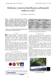
Example 1: For example, with n =25=4 2 +3 2 we
can construct the complex residue ring G25 isomorph to the
residue class ring Z25 according to 25 = (4 + 3i)(4 − 3i)
G25 = {z mod (4 + 3i),z ∈ Z25}
= {0, 1, 2, 3, −3i, −2+i, −1+i, i, 1 − i,
2+i, −1 − 2i, −2i, 1 − 2i, −1+2i, 2i,
1+2i, −2 − i, −1 − i, −i, 1 − i, 2 − i, 3i,
−3, −2, −1} . (8)
This complex constellation is also depicted in Fig. 1.
The complex residue class ring G25 is by definition an
additive group of Gaussian integers and a monoid under
multiplication. However, note that all elements of
G25 \{0, 5, 10, 15, 20} = G25 \{0, (−2+i), (−1−2i), (1+
2i), (2 − i)} have a multiplicative inverse. Furthermore,
similar to primitive elements of a finite field there exist
primitive roots that generate the ring G25 up to the
elements {5, 10, 15, 20}, i.e., the powers α i of any element
α ∈ {2, 3, 8, 12, 13, 17, 22, 23} generate the set
G25 \{0, 5, 10, 15, 20}.
Im
Re
Fig. 1. Complex constellation of the Gaussian integer ring G25.
Theorem 1 requires an integer m with a unique decomposition,
nevertheless there are non-prime integers with
multiple decompositions like 652 = a2 j + b2j = Πj ·
Π∗ j ; j =1,...,4 for which one may generalize the theorem
with multiple mappings to the Gaussian residue class ring
corresponding to the different decompositions.
IV. CODE CONSTRUCTION
A code C of length n over the ring Gm is a set of
codewords v = (v0,...,vn−1) with vi ∈ Gm. Wefirst
define some simple codes similar to codes over finite fields.
663
Then we use these simple codes to construct more powerful
codes based on well known code constructions. We only
consider codes where the sum of two codewords is also a
codeword. Hence, we have
d = min
v ′ ,v ′′ ∈C,v ′ =v ′′
dM(v ′ , v ′′ )= min
v∈C,v=0 wtM(v) (9)
for the minimum Mannheim distance d of the code C.
a) OMEC codes: Many code constructions presented
in [1] can be applied to Gaussian integer rings. Consider
for example the following one Mannheim error correcting
(OMEC) code. The parity check matrix of the code of
lengthupton = p(p − 1)/4 over the Gaussian residue
class ring G p 2 is constructed by the elements generated by
powers of a primitive root α, i.e.
H =(α 0 ,α 1 ,...,α n−1 ). (10)
Codewords are all vectors v =(v0,v1, ..., vn−1) with vi ∈
G p 2 for which Hv T = 0. A systematic encoding for the
information vector u is obtained by
v = (v0,u0,...,uk−1) with (11)
v0 = −α 1 u0 − α 2 u1 − ...− α n−1 uk−1.
Example 2: Using the ring G25 from example 1 with
p =5we can construct a code of length n =5with parity
check matrix
H =(1, 1+i, 2i, 1 − 2i, 3i)
where we have used the primitive root α = μ(8) = 1 + i.
This code has minimum Mannheim distance d =3and is
able to correct any Mannheim error of weight one, because
any single error from {1, −1,i,−i} will produce a different
syndrome.
b) Encoding binary information vectors: The mapping
of a binary information vector can be done by using
the Horner algorithm. We demonstrate the encoding in the
following example.
Example 3: The code from example 2 has dimension
k = n−1 =4and therefore has mk = 390625 codewords.
However, we can only map ⌊log2(mk )⌋ =18bits to each
codeword which results in a rate of R = 18
5 =3.6 bits per
symbol.
Let u (b) be the information vector in base b. Forexample,
we can interpret the vector
u (2) =(1, 0, 1, 1, 0, 0, 0, 0, 0, 0, 1, 0, 0, 1, 1, 0, 1, 0)
as the binary representation of the integer
u (10) =
17
j=0
uj2 j = 91149.
Using the Horner algorithm we can find the corresponding
representation in base 25
u (25) =(24, 20, 20, 5).
Using (6) we can map the elements of this vector to the
ring G25
u (4+3i) =(−1, 2 − i, 2 − i, −2+i).
Finally, with (11) we obtain the codeword
v =(1+i, −1, 2 − i, 2 − i, −2+i).

The encoding is systematic. Hence, using the inverse
mapping in (7) we can calculate the integer representation
u (10) of the information vector by 3 j=0 vj25j and the
binary representation using the Horner scheme again.
More powerful codes can be constructed by building
product codes or using the so-called Plotkin construction.
c) Product codes: The construction of product codes
was suggested by Peter Elias [6]. Let C1 and C2 be
(n1,k1,d1) and (n2,k2,d2) group codes over the Gaussian
integer ring Gm, respectively. We first encode k2 codewords
of the code C1 and store these codewords column wise into
the first k2 columns of a (n1 × n2)-matrix. Then we use
the code C2 n1-times to encode each row of this matrix.
The resulting code C has length n = n1n2 and dimension
k = k1k2.
Theorem 2: A product code over a Gaussian integer ring
has minimum Mannheim distance d ≥ d1d2.
Proof: According to (9) the minimum Mannheim
distance of the product code is equivalent to the minimum
weight of a non-zero codeword. A non-zero codeword has
at least one non-zero column. This column is a codeword
of the code C1 and has at least weight d1. However, each
non-zero element of this column results in a non-zero row.
Each non-zero row is a codeword of the code C2 and has
at least weight d2. Hence, a non-zero codeword has at least
d1 non-zero rows each with minimum weight d2.
Example 4: We can use the code from example 2 to
construct a product code of length n =25,dimensionk =
16, and minimum Mannheim distance d =9. This code
has rate R = 75
25 =2.96 bits per symbol.
d) Plotkin construction: Given two codes of length
n, the Plotkin construction can be used to obtain a code of
length 2n [7]. This construction works for linear and nonlinear
codes. Let C1 and C2 be two block codes of length
n1 = n2 over the Gaussian integer ring Gm. We construct
a code C by direct vector addition
C = {|v ′ |v ′ + v ′′ |, v ′ ∈C1, v ′′ ∈C2} (12)
Then C is also a block code over Gm. C has length n =2n1
and dimension k = k1 + k2, wherek1and k2 are the
dimensions of the codes C1 and C2, respectively.
Theorem 3: Code C resulting from the Plotkin construction
has minimum Mannheim distance d ≥ min{2d1,d2},
where d1 and d2 are the distances of the codes C1 and C2,
respectively.
The proof is very similar to the proof of the Plotkin
construction for binary codes in [12].
Example 5: We can use the code from example 2 as
code C1 and a repetition code C2 of length n2 = n1 =
5 to construct a Plotkin code of length n =2n1 =10.
A repetition code of length n2 is obtained by repeating
the information symbol u ∈Gm n2-times. The code has
dimension k2 =1and minimum Mannheim distance d2 =
n2. The resulting Plotkin code has dimension k =5and
minimum Mannheim distance d =5. Thus, this code has
rate R = 23
10 =2.3 bits per symbol.
V. DECODING
Let r = v + e denote the received vector where e is the
error vector. We first consider hard input decoding, i.e.,
we assume that ei ∈Gm. Reference [1] presents a simple
664
algebraic decoding algorithm for the code from example 2.
This code can correct any single error of Mannheim weight
one. For the algebraic decoding we calculate the syndrome
s = Hr T . We obtain the error location as l =log α smodn
and the error value el = Sα −l .
a) Hard input decoding of Plotkin codes: Now consider
the code resulting from the Plotkin construction as
in example 5. The code has minimum Mannheim distance
d =5and can correct any error up to Mannheim weight
two using the following decoding procedure. We assume
that the received vector is
r = |r ′ |r ′′ | = v + e
with e = |e ′ |e ′′ |, i.e., r ′ and e ′ denote the first halves of
the received vector and the error vector, r ′′ and e ′′ denote
the second halves, respectively.
Let t be the Mannheim weight of e. First,wedecodethe
vector r ′′ − r ′ = v ′′ + e ′′ − e ′ with respect to the repetition
code C2 using majority logic decoding, i.e., selecting the
symbol with the largest number of occurrences. Note that
the vector e ′′ − e ′ has Mannheim weight less or equal t.
Hence, C2 corrects all errors with t ≤⌊ d
2 ⌋.Letˆv′′ denote
the resulting estimate.
In the second step, we decode r ′ and r ′′ − ˆv ′′ with
respect to C1 which results in two estimates ˆv ′
1
and ˆv′
2 ,
respectively. Note that either e ′ or e ′′ has Mannheim weight
less or equal t/2. Therefore, either ˆv ′
1 or ˆv′ 2 is equal to the
transmitted codeword v ′ ∈C1 if t ≤⌊ d
2 ⌋.
To obtain the final estimate ˆv, we construct the code-
words |ˆv ′
1 |ˆv′
1 + ˆv′′ |, |ˆv ′
2 |ˆv′
2 + ˆv′′ | and select the one which
is closest to the received vector r.
b) Chase-type decoding: Chase algorithms [11] are
sub-optimum decoding algorithms for linear binary block
codes. This class of algorithms provides an efficient tradeoff
between error performance and decoding complexity.
They are based on conventional algebraic decoders. Where
the decoder generates a set of candidate codewords by
flipping some bit positions (test patterns) previous to the
algebraic decoding. The most likely codeword in this list
is chosen as the final estimate.
In the following we discuss low-complexity soft input
decoding procedures. In particular we show that the Chase
approach can be applied to codes over Gaussian integers.
Although the Chase-type algorithms are rather old, such
decoders are still highly relevant (see e.g. [13]).
Let r =(r0,...,rn−1) be the received vector after transmission
over an additive white Gaussian noise (AWGN)
channel. ˆri =[ri] denotes the hard-decision for the i-th
symbol, where [·] denotes rounding to the closest Gaussian
integer.
A Chase decoder generates a list of possible codewords,
which is used to calculate the estimated codeword by
comparing each codeword in the list with the received
vector r. In the case of binary codes, the list of codewords
is obtained by flipping bits in certain positions of the
received sequence. In the case of codes over Gaussian
integers, we add the symbols {1, −1,i,−i} to the most
unreliable symbol positions, i.e., to the positions with
largest weight wtM(ˆri − ri).
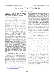
Simulation results for the code from example 2 are
depicted in Fig. 2. With hard input decoding the simple

OMEC code achieves a gain of approximately 2.5dB for a
symbol error rate of 10 −4 . Soft input decoding obtains an
additional gain of 0.5dB with a list of 13 codewords.
error rate
10 0
10 −1
10 −2
10 −3
10 −4
uncoded
hard
soft
12 13 14 15 16 17
E /N [dB]
S 0
18 19 20 21 22
Fig. 2. Simulation results for the OMEC code from example 2 over G25
for the AWGN channel.
This concept of soft decoding can also be applied to
Plotkin codes. Consider the hard input decoding described
in the previous paragraph. A simple soft input decoder
is obtained if, in the final decoding step, the closest
codeword is determined by using the Euclidean distance.
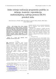
Corresponding simulation results for the code from example
5 are depicted in Fig. 3. In this case, hard input
decoding achieves a gain close to 4dB for a symbol error
rate of 10 −4 . With this simple soft input decoding we
obtain an additional gain of 0.5dB with only two candidate
codewords.
A larger list can be obtained by using list decoding for
the constituent codes. In the first decoding step, we can
use soft input maximum-likelihood decoding to decode the
repetition code and obtain a list L2 of codewords from code
C2 by adding the symbols {1, −1,i,−i} to the maximumlikelihood
estimate. In the second step, we use Chase
decoding for r ′ . Furthermore, we use Chase decoding for
r ′′ − ˆv ′′
l
for each element ˆv′′
l ∈L2 of the list. This results
in a list L1 of codewords from the code C1.
Finally, we construct all possible codewords
|ˆv ′ j|ˆv ′ j + ˆv ′′
l |, ˆv ′ j ∈L1, ˆv ′′
l ∈L2
and select the one which is closest to the received vector.
VI. CONCLUSIONS
In this work we have considered codes over Gaussian
integer rings. All constructions are possible for Gaussian
integer fields as well as for rings. Gaussian integer rings
extend the possible complex signal constellations for codes
over Gaussian integers. We have shown that binary information
vectors can easily be encoded to such codes.
Most previous publications on codes over Gaussian
integers considered only hard input or optimum maximumlikelihood
decoding (e.g. [1]-[5]). However, maximumlikelihood
decoding is only feasible for small signal constellations
and short codes. We have shown that lowcomplexity
soft input decoding is possible by using a
665
error rate
10 0
10 −1
10 −2
10 −3
10 −4
uncoded
hard
soft
12 13 14 15 16 17
E /N [dB]
S 0
18 19 20 21 22
Fig. 3. Simulation results for the Plotkin code from example 5 over G25
for the AWGN channel.
Chase-type algorithm [11]. Likewise, the recursive structure
of the Plotkin construction can be exploited for
decoding similar to the sub-optimum decoding of Reed-
Muller codes [8], [10], [14].
REFERENCES
[1] K. Huber, Codes over Gaussian integers, Information Theory, IEEE
Transactions on, Volume 40, Issue 1, Jan. 1994 Page(s):207 - 216
Information Theory, IEEE Transactions on, Volume: 41 , Issue 5,
1995 , Page(s): 1512 - 1517
[2] Xue-dong Dong, Cheong Boon Soh, E. Gunawan, Li-zhong Tang,
Groups of algebraic integers used for coding QAM signals, Information
Theory, IEEE Transactions on, Volume 44, Issue 5, Sept.
1998 Page(s):1848 1860
[3] M. Bossert, E.M. Gabidulin, P. Lusina, Space-time codes based on
Gaussian integers, inInformation Theory, 2002. Proceedings. 2002
IEEE International Symposium on, 2002 Page(s):273 - 421
[4] P. Lusina, S. Shavgulidze, M. Bossert, Space - time block factorisation
codes over Gaussian integers, IEE Proceedings, Volume 151,
Issue 5, 24 Oct. 2004 Page(s):415 - 421
[5] J. Rifa, Groups of complex integers used as QAM signals,
[6] P. Elias, Error-free coding, IRE Trans. on Inform. Theory, PGIT-4:
29-37, 1954.
[7] Morris Plotkin, Binary Codes with Specified Minimum Distance,
IRE Transactions on Inform. Theory, Vol. 6, pp. 445-450, 1960
[8] G. Schnabl, M. Bossert, Soft-Decision Decoding of Reed-Muller
Codes as Generalized Multiple Concatenated Codes, Information
Theory, IEEE Transactions on, Vol. IT-41, pp. 304-308, 1995
[9] H. Scheid and A. Frommer, ”Number theory”, (German), (Elsevier-
Spektrum Akademiv publishing, 2007).
[10] N. Stolte, Rekursive Codes mit der Plotkin-Konstruktion und ihre
Decodierung, [Dissertation], TU Darmstadt, 2002
[11] D. Chase, A class of algorithms for decoding block codes with
channel measurement information, IEEE Trans. Inform. Theory,
Vol. 18, pp. 170- 182, Jan. 1972.
[12] M. Bossert, Channel Coding for Telecommunications, John Wiley
& Sons, 1999
[13] C. Argon, S.W. McLaughlin, and T. Souvignier, Iterative application
of the Chase algorithm on Reed-Solomon product codes, Proceedings
IEEE ICC 2001, pp. 320-324, 2001.
[14] I. Dumer , G. Kabatiansky, C. Tavernier, List decoding of Reed-
Muller codes up to the Johnson bound with almost linear complexity,
Proceedings Information Theory, 2006 IEEE International
Symposium on , pp.138-142, 9-14 July 2006