Compatibility of induction methods for mantle ... - MTNet - DIAS
Compatibility of induction methods for mantle ... - MTNet - DIAS Compatibility of induction methods for mantle ... - MTNet - DIAS
B03101 face inhomogeneities. The main difficulty, in addition to the selection of the appropriate impedance relationships for the modeling, is the complicated numeric simulation technique required for the generalized HSG method. We believe that this study will help to achieve higher confidence in the results of mantle soundings and to achieve as broad a depth range of investigation of the mantle as possible. 2. Impedance Relationships for Modeling 2.1. Magnetotelluric Approach [5] The linear MT impedance relationship, considered in the Tikhonov‐Cagniard model [Cagniard, 1953] for a layered medium, follows also from Rytov’s impedance boundary conditions (IBC) for the “weakly” inhomogeneous case [Rytov, 1940; Senior and Volakis, 1995]. An approximate form of the Rytov’s infinite power series with scalar impedance and neglected terms of higher than first order of the spatial derivatives is known as the Leontovich’s IBC [Leontovich, 1948; Senior and Volakis, 1995]. Leontovich’s scalar relation, generalized for anisotropic media [Landau and Lifshic, 1959; Senior and Volakis, 1995], has been applied by Berdichevsky and Cantwell [Berdichevsky et al., 1997] for MT soundings and can be written in the vector form [Guglielmi, 2009]: E Z ðHnÞ: ð1Þ [6] Here Z is the impedance tensor with components Zij(w, r) that depend on the angular frequency w and the coordinates of the position vector r at the boundary between conductive (earth) and resistive (air) media; Et and Ht are the tangential complex Fourier amplitudes of the electric and magnetic fields, respectively; n is a unit vector normal to the boundary. The traditional relationship (1) will be used in the modeling of the MT method, though the generalized one on a closed surface has also been derived by Shuman [1999, 2003, 2007]. 2.2. Magnetovariational Approach [7] The generalized HSG method also follows from Rytov’s IBC in an approximate form under the same condition for the spatial derivatives. The generalized HSG approach was first written out in its explicit form by Guglielmi and Gokhberg [1987], which we show in the form Hz ð Þ 1 ½ZdivH ð ÞþHðgradZÞŠ; ð2Þ i! 0 VOZAR AND SEMENOV: INDUCTION METHODS FOR MANTLE SOUNDINGS B03101 where Z(w, r) is the scalar impedance as defined by Guglielmi [2009]; m0 is the magnetic permeability of the free space; i is the imaginary unit and Hz is the Fourier amplitude of the magnetic component orthogonal to the Earth’s surface. The sign in (2) depends on the chosen reference system. Rytov’s IBC, derived for radio wave periods, is valid for cases characterized by large values of thewavenumber[Guglielmi, 1984]oroftherefractive index [Senior and Volakis, 1995]. These and several other requirements of Rytov’s theory are correct for short‐period subsurface soundings but they are incorrect for the low 2of9 frequencies employed for deep induction sounding of the mantle. [8] A second approach to the generalized HSG sounding method was suggested by Schmucker [2003, 2008] and is represented as the combination of the traditional HSG method and the Wise‐Parkinson relationship with tippers: Bz ¼ C ð! Þ f@Bnx=@x þ @Bny=@ygþzHBnx þ zDBny þ Bz; ð3Þ where C(w) =Z(w)/íwm0 is the scalar C‐response, zH and zD are the transfer functions (tippers) and dB z denotes noise. The amplitudes of the observed magnetic field components are subdivided into “normal” (with subscript n) and “anomalous” parts. While the observed vertical component B z includes both the normal and anomalous parts, the anomalous horizontal field components are neglected in Schmucker’s approach, which provides the main distinction from other generalized MV approaches. Examples of applying this approach (3) to real data are also presented by Schmucker [2003, 2008]. [9] A third approach to MV soundings is based on the vectoral impedance boundary conditions with two scalar impedances z(w, r) and x(w, r) on a closed surface [Aboul‐ Atta and Boerner, 1975], expanded for the MV method by Shuman and Kulik [2002]: i! 0Hr ¼ divH þ H grad þ * divH * þ H * grad * : ð4Þ where Hr is the radial component on the surface of a spherical model, the asterisk indicates the complex conjugate. Shuman’s approach (4) coincides with equation (2) if the impedance x* =0[Shuman, 2003, 2007]. In case that gradz = 0 for a laterally homogeneous medium and the expression represents the common HSG method: i! 0Hr ¼ m divH : ð5Þ [10] Equation (5) will be used in our modeling in sections 3 and 4. Assuming the pure P 1 0 mode for a linearly polarized Dst source at ultralong periods, the expression (5) can be transformed to the relationship of the GDS method [Olsen, 1998] written out in geomagnetic spherical coordinates: i! 0H g r ¼ g m 2H g =R tg g o : ð6Þ where zm g (w) is the impedance of the GDS method, R is the Earth’s radius, and o g is the colatitude of the measurement point. Expression (6) will be used in our modeling. [11] In practice, all the methods considered above for taking soundings of a medium are applied without a priori knowledge of the medium properties and structure. While theoretically the impedances for all methods should be identical in the case of laterally homogeneous media, in practice it proves almost impossible to locate test sites in which the subsurface is homogeneous. Therefore we use a forward modeling approach to allow us to compare the impedances from each method over known subsurface structures using known fields. We follow the simplest approach for the modeling of the generalized HSG method by using the differential relation (2) as an approximate form of relation (4). We simulate the observed field components on a sphere for a
B03101 number of different structural models without the separation of the fields into “normal” and “anomalous” parts. 3. Method of Numerical Simulation VOZAR AND SEMENOV: INDUCTION METHODS FOR MANTLE SOUNDINGS B03101 Figure 1. Schematic model of the Earth’s conductivity structure assumed in our modeling. The conductances of outer surface shell are used in the final model in Figure 6. In all other models the variable conductance outer shell was replaced with a constant conductance shell (20 S). [12] Forward modeling of the electromagnetic fields excited by ionospheric and magnetospheric sources is carried out on the globe with the alignment of the geographical and geomagnetic reference systems, using the program elaborated by Kuvshinov et al. [2005]. The impedances for the MT and “classic” MV methods can be calculated directly from the modeled field components using relations (1), (5), and (6). [13] The assumed layered Earth structure includes a step in the highly conductive layer of the mantle as shown in Figure 1. The step structure is characterized by a sharp, but not discontinuous, jump in the conductive layer (see the inset in Figure 1), which allows current flow through the structure and therefore maximizes the effects on the fields induced by this mantle inhomogeneity. Spatial distributions of all field components have been computed on the globe at a grid interval of 1° × 1° for a period range from 10 min to 4096 days. Three spherical models were used for testing the methods: 2‐D and 3‐D spherical models with a homogeneous surface conductance of 20S assumed, and one 3‐D spherical model where a realistic surface shell conductance [Vozar et al., 2006] has been taken into consideration (Figure 1). [14] There are no magnetotelluric plane wave sources for spherical models. But since we work only with impedances, it is sufficient to use horizontal (tangential) source fields that locally depend linearly on the horizontal coordinates [Berdichevsky and Dmitriev, 2008]. One can excite the 3of9 modeled Earth by two polarizations of the source field and thus obtain the tensor of impedances. One requires three polarizations (instead of two in the plane case) in order to avoid the singularities arising globally because of the change of signs of the cos and sin functions. A spherical analog for the “plane wave” source used in the MT method can be approximated by three orthogonal sources of a ring current type. A single ring current is sufficient as a source for modeling in the case of the MV methods based on the expressions mentioned above ((2), (3), (5), and (6)). [15] The impedances of the generalized HSG method cannot be determined directly from the modeled magnetic field components. Relation (4) with x* = 0 has been considered as a differential equation with unknown scalar impedance: ðH =RÞ @ m=@ þ H’= ðRsin Þ @ m=@’ þ m @ðHsin Þ=@ þ @H’=@’ = ðRsin Þ i! 0Hr ¼ 0: [16] The general solution of equation (7) on the surface of a sphere is obtained for spherical 3‐D inhomogeneous structures by using a numerical finite difference method: A simple five‐point stencil discretization was applied to derive the central finite difference approximations of derivatives at the spherical grid points. As a result, a system of linear equations (with a small modification of the stencil to an asymmetric one on the grid boundary) has been obtained with the impedances as unknown parameters at all grid points. ð7Þ
- Page 1: Click Here for Full Article Compati
- Page 5 and 6: B03101 have only one component A. T
- Page 7 and 8: B03101 VOZAR AND SEMENOV: INDUCTION
- Page 9: B03101 VOZAR AND SEMENOV: INDUCTION
B03101<br />
number <strong>of</strong> different structural models without the separation<br />
<strong>of</strong> the fields into “normal” and “anomalous” parts.<br />
3. Method <strong>of</strong> Numerical Simulation<br />
VOZAR AND SEMENOV: INDUCTION METHODS FOR MANTLE SOUNDINGS B03101<br />
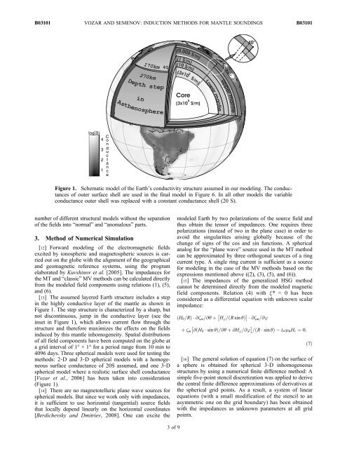
Figure 1. Schematic model <strong>of</strong> the Earth’s conductivity structure assumed in our modeling. The conductances<br />
<strong>of</strong> outer surface shell are used in the final model in Figure 6. In all other models the variable<br />
conductance outer shell was replaced with a constant conductance shell (20 S).<br />
[12] Forward modeling <strong>of</strong> the electromagnetic fields<br />
excited by ionospheric and magnetospheric sources is carried<br />
out on the globe with the alignment <strong>of</strong> the geographical<br />
and geomagnetic reference systems, using the program<br />
elaborated by Kuvshinov et al. [2005]. The impedances <strong>for</strong><br />
the MT and “classic” MV <strong>methods</strong> can be calculated directly<br />
from the modeled field components using relations (1), (5),<br />
and (6).<br />
[13] The assumed layered Earth structure includes a step<br />
in the highly conductive layer <strong>of</strong> the <strong>mantle</strong> as shown in<br />
Figure 1. The step structure is characterized by a sharp, but<br />
not discontinuous, jump in the conductive layer (see the<br />
inset in Figure 1), which allows current flow through the<br />
structure and there<strong>for</strong>e maximizes the effects on the fields<br />
induced by this <strong>mantle</strong> inhomogeneity. Spatial distributions<br />
<strong>of</strong> all field components have been computed on the globe at<br />
a grid interval <strong>of</strong> 1° × 1° <strong>for</strong> a period range from 10 min to<br />
4096 days. Three spherical models were used <strong>for</strong> testing the<br />
<strong>methods</strong>: 2‐D and 3‐D spherical models with a homogeneous<br />
surface conductance <strong>of</strong> 20S assumed, and one 3‐D<br />
spherical model where a realistic surface shell conductance<br />
[Vozar et al., 2006] has been taken into consideration<br />
(Figure 1).<br />
[14] There are no magnetotelluric plane wave sources <strong>for</strong><br />
spherical models. But since we work only with impedances,<br />
it is sufficient to use horizontal (tangential) source fields<br />
that locally depend linearly on the horizontal coordinates<br />
[Berdichevsky and Dmitriev, 2008]. One can excite the<br />
3<strong>of</strong>9<br />
modeled Earth by two polarizations <strong>of</strong> the source field and<br />
thus obtain the tensor <strong>of</strong> impedances. One requires three<br />
polarizations (instead <strong>of</strong> two in the plane case) in order to<br />
avoid the singularities arising globally because <strong>of</strong> the<br />
change <strong>of</strong> signs <strong>of</strong> the cos and sin functions. A spherical<br />
analog <strong>for</strong> the “plane wave” source used in the MT method<br />
can be approximated by three orthogonal sources <strong>of</strong> a ring<br />
current type. A single ring current is sufficient as a source<br />
<strong>for</strong> modeling in the case <strong>of</strong> the MV <strong>methods</strong> based on the<br />
expressions mentioned above ((2), (3), (5), and (6)).<br />
[15] The impedances <strong>of</strong> the generalized HSG method<br />
cannot be determined directly from the modeled magnetic<br />
field components. Relation (4) with x* = 0 has been<br />
considered as a differential equation with unknown scalar<br />
impedance:<br />
ðH =RÞ<br />
@ m=@ þ H’= ðRsin Þ @ m=@’<br />
þ m @ðHsin Þ=@ þ @H’=@’ = ðRsin Þ i! 0Hr ¼ 0:<br />
[16] The general solution <strong>of</strong> equation (7) on the surface <strong>of</strong><br />
a sphere is obtained <strong>for</strong> spherical 3‐D inhomogeneous<br />
structures by using a numerical finite difference method: A<br />
simple five‐point stencil discretization was applied to derive<br />
the central finite difference approximations <strong>of</strong> derivatives at<br />
the spherical grid points. As a result, a system <strong>of</strong> linear<br />
equations (with a small modification <strong>of</strong> the stencil to an<br />
asymmetric one on the grid boundary) has been obtained<br />
with the impedances as unknown parameters at all grid<br />
points.<br />
ð7Þ


