P. Schmoldt, PhD - MTNet - DIAS

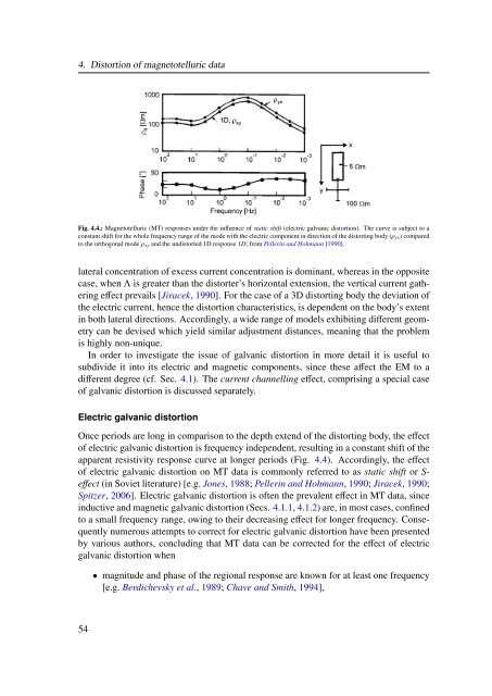
4. Distortion of magnetotelluric data
Fig. 4.4.: Magnetotelluric (MT) responses under the influence of static shift (electric galvanic distortion). The curve is subject to a
constant shift for the whole frequency range of the mode with the electric component in direction of the distorting body (ρyx) compared
to the orthogonal mode ρxy and the undistorted 1D response 1D; from Pellerin and Hohmann [1990].
lateral concentration of excess current concentration is dominant, whereas in the opposite
case, when Λ is greater than the distorter’s horizontal extension, the vertical current gathering
effect prevails [Jiracek, 1990]. For the case of a 3D distorting body the deviation of
the electric current, hence the distortion characteristics, is dependent on the body’s extent
in both lateral directions. Accordingly, a wide range of models exhibiting different geometry
can be devised which yield similar adjustment distances, meaning that the problem
is highly non-unique.
In order to investigate the issue of galvanic distortion in more detail it is useful to
subdivide it into its electric and magnetic components, since these affect the EM to a
different degree (cf. Sec. 4.1). The current channelling effect, comprising a special case
of galvanic distortion is discussed separately.
Electric galvanic distortion
Once periods are long in comparison to the depth extend of the distorting body, the effect
of electric galvanic distortion is frequency independent, resulting in a constant shift of the
apparent resistivity response curve at longer periods (Fig. 4.4). Accordingly, the effect
of electric galvanic distortion on MT data is commonly referred to as static shift or Seffect
(in Soviet literature) [e.g. Jones, 1988; Pellerin and Hohmann, 1990; Jiracek, 1990;
Spitzer, 2006]. Electric galvanic distortion is often the prevalent effect in MT data, since
inductive and magnetic galvanic distortion (Secs. 4.1.1, 4.1.2) are, in most cases, confined
to a small frequency range, owing to their decreasing effect for longer frequency. Consequently
numerous attempts to correct for electric galvanic distortion have been presented
by various authors, concluding that MT data can be corrected for the effect of electric
galvanic distortion when
54
• magnitude and phase of the regional response are known for at least one frequency
[e.g. Berdichevsky et al., 1989; Chave and Smith, 1994],