P. Schmoldt, PhD - MTNet - DIAS
P. Schmoldt, PhD - MTNet - DIAS P. Schmoldt, PhD - MTNet - DIAS
2. Sources for magnetotelluric recording Fig. 2.3.: A schematic view of the magnetosphere; from Potemra [1984]. Tab. 2.1.: Classification of geomagnetic variations sorted by their characteristic time τ, after Schmucker [1985] with updates for the ULF frequency bands from McPherron [2005] and characterisation of the solar daily variation in the equatorial region of the day-side as equatorial electrojet (EEJ). τ: Fundamental period for regular variations, period range for irregular variations. A: Peak-to-peak amplitude or maximum departure from undisturbed level. If a significant dependence on latitudes exists, different values are quoted for auroral zone (a), mid-latitudes (m), low-latitudes (l) and the dip equator region on the day side (dd). ERC: Equatorial ring current in the radiation belt of the magnetosphere. 10 Type Symbol τ A (nT) Source Ultralong periodic variation Solar cycle variations 11 years 20 ERC modulation by sunspot cycle Annual variations 1 year 5 Ionospheric sources Semi-annual variation 6 month 5 ERC modulation within the Earth’s orbit around the sun Smoothed storm-time variations storm time-dependent part Dst 2 - 27 d 100 disturbance local time inequality DS 12 - 24 h 100 Solar daily variations on quiet days equatorial electrojet enhanced on disturbed days Sq EEJ SD 1 d 1 d 1 d 30 - 60 (m,l) 60 - 120 (dd) 1 - 20 Ionospheric current loops on day-side sectors of both hemispheres Lunar daily variations L 1 lunar daya 1 - 3 Dual ionospheric current loops on both hemispheres Continued on Next Page. . .
Tab. 2.1 – Continued 2.2. Electric currents in the magnetosphere Type Symbol τ A (nT) Source Polar magnetic storms and short-lived substorms Polar (or auroral) centre of disturbance in the night-time auroral zone with correlated irregular variations in low latitudes DP1 10 m - 2 h DP2 10 m - 2 h Special effects in connection to polar magnetic storms bays (substorms as observed in mid latitudes) b 30 m -2 h Sudden storm commencement 1000 (a) 100 (m,l) 100 (a) 10 (m,l) 100 (d,d) 20 - 100 (a,m) 5 - 25 (l) electrojet PEJ in the ionosphere with connecting field-aligned currents to plasma regions of the magnetosphere see DP1 ssc 2 - 5 m 10 - 100 m Impact of intense solar particle stream on magnetopause Solar flare effect sfe 10 - 20 m 10 Short-lived enhancement of Sq currents in the ionosphere Ultralow frequency waves (Pulsations) regular continuous pulsations irregular transient pulsations Very low frequency emissions, including whistlers ULF (P) 0.2 - 600 s Pc5 150 - 600 s 100 (a) 10 (m) Pc4 45 - 150 s 2 Pc3 10 - 45 s 0.5 Pc3 5 - 10 s 0.5 Pc1 0.2 - 5 s 1 Pi2 45 - 150 s 1 Pi1 1 - 45 s 1 VLF 10 −5 − 10 −3 s 2.2.1. Ultralong periodic variation Standing and propagating hydromagnetic waves in the magnetosphere In this Section geomagnetic variations with extremely long periods are examined that are not directly related to conventional MT measurements, which are, for logistic reason, usually limited to a duration of a few months or less. Signals of such ultralong variations are more suitable for studies using magnetovariational (MV) datasets, recorded at stationary observatories that provide time series of sufficient length. However, the results of those MV studies can be used to compare findings of MT methods and help to predict structures at greater depth, which in turn can aid interpretation of MT studies. a Schmucker [1985] assigns the Lunar daily variations to have a fundamental period of 1 d but as the determining value is the time that it takes the Moon to orbit the Earth this variation has a period of around 24 h 50 m (1 lunar day) instead, e.g. Merrill and McElhinny [1983], p.53; National Oceanic and Atmospheric Administration (NOAA) [2010]. 11
- Page 1: Multidimensional isotropic and anis
- Page 4 and 5: Contents 2.3. Deviation from plane
- Page 6 and 7: Contents 8.3. Inversion of 3D model
- Page 9 and 10: List of Figures 2.1. Amplitude of t
- Page 11 and 12: List of Figures 4.17. Visual repres
- Page 13 and 14: List of Figures 8.2. Ambient noise
- Page 15 and 16: List of Figures 10.10.RMS misfit va
- Page 17: List of Figures A.15.Result of anis
- Page 20 and 21: List of Tables xviii 5.5. Parameter
- Page 22 and 23: List of Acronyms FE finite element
- Page 25 and 26: List of Symbols Below is a list of
- Page 27 and 28: Symbol SI unit Denotation φ · pha
- Page 29: Abstract The Tajo Basin and Betic C
- Page 32 and 33: Publications Poster presentations x
- Page 34 and 35: Acknowledgements Team, namely Colin
- Page 37 and 38: Introduction 1 The Iberian Peninsul
- Page 39 and 40: ections from enhanced one-dimension
- Page 41: Part I Theoretical background of ma
- Page 44 and 45: 2. Sources for magnetotelluric reco
- Page 48 and 49: 2. Sources for magnetotelluric reco
- Page 50 and 51: 2. Sources for magnetotelluric reco
- Page 52 and 53: 2. Sources for magnetotelluric reco
- Page 54 and 55: 2. Sources for magnetotelluric reco
- Page 56 and 57: 2. Sources for magnetotelluric reco
- Page 58 and 59: 2. Sources for magnetotelluric reco
- Page 60 and 61: 2. Sources for magnetotelluric reco
- Page 62 and 63: 2. Sources for magnetotelluric reco
- Page 64 and 65: 2. Sources for magnetotelluric reco
- Page 67 and 68: Mathematical description of electro
- Page 69 and 70: yields 3.2. Deriving magnetotelluri
- Page 71 and 72: 3.2. Deriving magnetotelluric param
- Page 73 and 74: 3.3. Magnetotelluric induction area
- Page 75 and 76: Depth d s d 1 d 2 d n-2 d n-1 t 1 t
- Page 77 and 78: 3.4. Boundary conditions materials
- Page 79 and 80: 3.5. The influence of electric perm
- Page 81 and 82: 3.5. The influence of electric perm
- Page 83 and 84: 3.5. The influence of electric perm
- Page 85 and 86: Distortion of magnetotelluric data
- Page 87 and 88: 4.1. Types of distortion Fig. 4.1.:
- Page 89 and 90: 4.1. Types of distortion Fig. 4.3.:
- Page 91 and 92: J s 0 s 0 4.1. Types of distortion
- Page 93 and 94: 4.1. Types of distortion Fig. 4.7.:
- Page 95 and 96: Scale Type Terminology Example Atom
2. Sources for magnetotelluric recording<br />
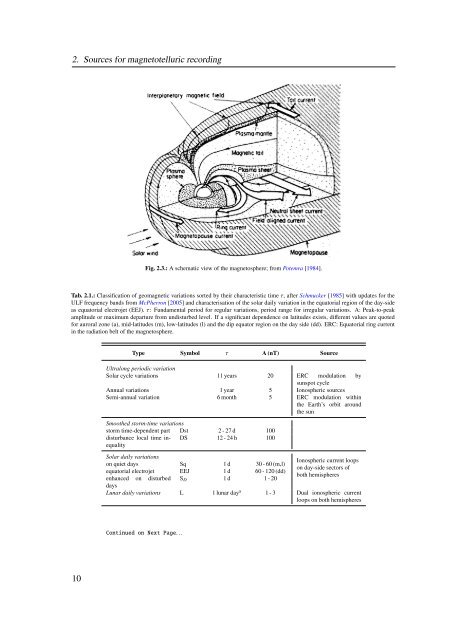
Fig. 2.3.: A schematic view of the magnetosphere; from Potemra [1984].<br />
Tab. 2.1.: Classification of geomagnetic variations sorted by their characteristic time τ, after Schmucker [1985] with updates for the<br />
ULF frequency bands from McPherron [2005] and characterisation of the solar daily variation in the equatorial region of the day-side<br />
as equatorial electrojet (EEJ). τ: Fundamental period for regular variations, period range for irregular variations. A: Peak-to-peak<br />
amplitude or maximum departure from undisturbed level. If a significant dependence on latitudes exists, different values are quoted<br />
for auroral zone (a), mid-latitudes (m), low-latitudes (l) and the dip equator region on the day side (dd). ERC: Equatorial ring current<br />
in the radiation belt of the magnetosphere.<br />
10<br />
Type Symbol τ A (nT) Source<br />
Ultralong periodic variation<br />
Solar cycle variations 11 years 20 ERC modulation by<br />
sunspot cycle<br />
Annual variations 1 year 5 Ionospheric sources<br />
Semi-annual variation 6 month 5 ERC modulation within<br />
the Earth’s orbit around<br />
the sun<br />
Smoothed storm-time variations<br />
storm time-dependent part Dst 2 - 27 d 100<br />
disturbance local time inequality<br />
DS 12 - 24 h 100<br />
Solar daily variations<br />
on quiet days<br />
equatorial electrojet<br />
enhanced on disturbed<br />
days<br />
Sq<br />
EEJ<br />
SD<br />
1 d<br />
1 d<br />
1 d<br />
30 - 60 (m,l)<br />
60 - 120 (dd)<br />
1 - 20<br />
Ionospheric current loops<br />
on day-side sectors of<br />
both hemispheres<br />
Lunar daily variations L 1 lunar daya 1 - 3 Dual ionospheric current<br />
loops on both hemispheres<br />
Continued on Next Page. . .


