P. Schmoldt, PhD - MTNet - DIAS
P. Schmoldt, PhD - MTNet - DIAS P. Schmoldt, PhD - MTNet - DIAS
4. Distortion of magnetotelluric data Parameter Geoelectrical application I1 = (ξ 2 4 + ξ2 1 )1/2 I2 = (η 2 4 + η2 1 )1/2 I3 = (ξ 2 2 + ξ2 3 )1/2 /I1 }2D anisotropy I4 = (η 2 2 + η2 3 )1/2 /I2 I5 = (ξ4η1 + ξ1η4)/(I1I2) I6 = (ξ4η1 − ξ1η4)/(I1I2) I7 = (d41 − d23)/Q QW = [(d12 − d34) 2 + (d13 + d24) 2 ] 1/2 1D magnitude and phase of the geoelectric resistivity (Eq. 4.47 and 4.48) }Galvanic distortion Tab. 4.3.: The seven independent (I1 - I7) plus one dependent parameter (Q) defined by Weaver et al. [2000] to describe the magnetotelluric (MT) impedance tensor and its distortion. Each of the parameters is associated with a certain geological setup, and subsurface characteristics in terms of dimensionality and distortion can be derived from the values of these parameters; see Table 4.4 for details about the relation between parameter values and subsurface dimensionality. Relation of ξ, η, and d with the MT impedance tensor are given in Equations 4.42 – 4.46 Values Dimensionality I3 = I4 = I5 = I6 = 0; I7 = 0 or QW = 0 1D I3 0 or I4 0; I7 = 0 or QW = 0 2D I3 0 or I4 0; I5 0, I7 = 0 3D/2Dtwist (only twist) I3 0 or I4 0; I5 0, I7 : undefined I6 0 3D/2D1D (non-recoverable strike direction) galvanic distortion over a 1D or 2D structure 3D/2D general case of galvanic distortion over a 2D structure I7 0 3D (affected or not by galvanic distortion) Tab. 4.4.: The dimensionality of the subsurface derived from the parameters defined by Weaver et al. [2000], after [Martí et al., 2005] and [Martí, 2007]. given via a Mohr circle diagram with the rotated impedance tensor elements Zxx and Zxy forming the x and y-axis (Fig. 4.16). Assumptions about the subsurface dimensionality can be made with the values WAL parameters (Tab. 4.4). Due to noise in a real data set, the parameters will not exhibit values of exactly zero and threshold values need to be introduced. Certainly, threshold values have significant influence onto the derived dimensionality and have to be chosen carefully. In their publication, Weaver et al. [2000] propose a value of 0.1 as tolerance level for all parameters, whereas Martí et al. [2009b] use default threshold values of 0.15 for the independent parameters and 0.1 for QW in their program WALDIM, the latter being an implementation of the theory by Weaver et al. [2000]. Information about the apparent resistivity and phase of the related 1D subsurface can be obtained from invariants I1 and I2 giving an approximate idea about the conductivity 72
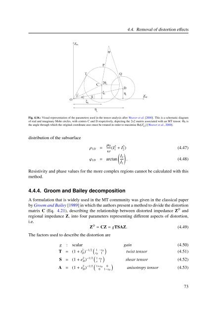
4.4. Removal of distortion effects Fig. 4.16.: Visual representation of the parameters used in the tensor analysis after Weaver et al. [2000]. This is a schematic diagram of real and imaginary Mohr circles, with centres C and D respectively, depicting the 2x2 matrix associated with an MT tensor. Θ0 is the angle through which the original coordinate axes must be rotated in order to maximise Re[Z ′ 12 ] [Weaver et al., 2000]. distribution of the subsurface ρ1D = µ0 ω (I2 1 ϕ1D = arctan + I2 2 ) (4.47) I2 . (4.48) Resistivity and phase values for the more complex regions cannot be calculated with this method. 4.4.4. Groom and Bailey decomposition A formulation that is widely used in the MT community was given in the classical paper by Groom and Bailey [1989] in which the authors present a method to divide the distortion matrix C (Eq. 4.21), describing the relationship between distorted impedance Z D and regional impedance Z, into four parameters representing different aspects of distortion, i.e. Z D = CZ = gTSAZ. (4.49) The factors used to describe the distortion are I1 g : scalar gain (4.50) T = (1 + t 2 D) −1/2 1 −tD tD 1 twist tensor (4.51) S = (1 + e 2 D) −1/2 1 eD e 1 shear tensor (4.52) A = (1 + s 2 D) −1/2 1+sD 0 0 anisotropy tensor (4.53) 1−sD 73
- Page 58 and 59: 2. Sources for magnetotelluric reco
- Page 60 and 61: 2. Sources for magnetotelluric reco
- Page 62 and 63: 2. Sources for magnetotelluric reco
- Page 64 and 65: 2. Sources for magnetotelluric reco
- Page 67 and 68: Mathematical description of electro
- Page 69 and 70: yields 3.2. Deriving magnetotelluri
- Page 71 and 72: 3.2. Deriving magnetotelluric param
- Page 73 and 74: 3.3. Magnetotelluric induction area
- Page 75 and 76: Depth d s d 1 d 2 d n-2 d n-1 t 1 t
- Page 77 and 78: 3.4. Boundary conditions materials
- Page 79 and 80: 3.5. The influence of electric perm
- Page 81 and 82: 3.5. The influence of electric perm
- Page 83 and 84: 3.5. The influence of electric perm
- Page 85 and 86: Distortion of magnetotelluric data
- Page 87 and 88: 4.1. Types of distortion Fig. 4.1.:
- Page 89 and 90: 4.1. Types of distortion Fig. 4.3.:
- Page 91 and 92: J s 0 s 0 4.1. Types of distortion
- Page 93 and 94: 4.1. Types of distortion Fig. 4.7.:
- Page 95 and 96: Scale Type Terminology Example Atom
- Page 97 and 98: 4.1. Types of distortion the use of
- Page 99 and 100: 4.2. Dimensionality Fig. 4.12.: The
- Page 101 and 102: 1D 2D local 3D/1D 3D/2D regional 4.
- Page 103 and 104: 4.3. General mathematical represent
- Page 105 and 106: 4.4. Removal of distortion effects
- Page 107: Parameter Geoelectrical application
- Page 111 and 112: 4.4.5. Caldwell-Bibby-Brown phase t
- Page 113 and 114: 4.4. Removal of distortion effects
- Page 115: Method Applicability Swift angle 2D
- Page 118 and 119: 5. Earth’s properties observable
- Page 120 and 121: 5. Earth’s properties observable
- Page 122 and 123: 5. Earth’s properties observable
- Page 124 and 125: 5. Earth’s properties observable
- Page 126 and 127: 5. Earth’s properties observable
- Page 128 and 129: 5. Earth’s properties observable
- Page 130 and 131: 5. Earth’s properties observable
- Page 132 and 133: 5. Earth’s properties observable
- Page 134 and 135: 5. Earth’s properties observable
- Page 136 and 137: 5. Earth’s properties observable
- Page 138 and 139: 5. Earth’s properties observable
- Page 140 and 141: 5. Earth’s properties observable
- Page 142 and 143: 6. Using magnetotellurics to gain i
- Page 144 and 145: 6. Using magnetotellurics to gain i
- Page 146 and 147: 6. Using magnetotellurics to gain i
- Page 148 and 149: 6. Using magnetotellurics to gain i
- Page 150 and 151: 6. Using magnetotellurics to gain i
- Page 152 and 153: 6. Using magnetotellurics to gain i
- Page 154 and 155: 6. Using magnetotellurics to gain i
- Page 156 and 157: 6. Using magnetotellurics to gain i
4.4. Removal of distortion effects<br />
Fig. 4.16.: Visual representation of the parameters used in the tensor analysis after Weaver et al. [2000]. This is a schematic diagram<br />
of real and imaginary Mohr circles, with centres C and D respectively, depicting the 2x2 matrix associated with an MT tensor. Θ0 is<br />
the angle through which the original coordinate axes must be rotated in order to maximise Re[Z ′ 12 ] [Weaver et al., 2000].<br />
distribution of the subsurface<br />
ρ1D = µ0<br />
ω (I2 1<br />
ϕ1D = arctan<br />
+ I2 2 ) (4.47)<br />
<br />
I2<br />
. (4.48)<br />
Resistivity and phase values for the more complex regions cannot be calculated with this<br />
method.<br />
4.4.4. Groom and Bailey decomposition<br />
A formulation that is widely used in the MT community was given in the classical paper<br />
by Groom and Bailey [1989] in which the authors present a method to divide the distortion<br />
matrix C (Eq. 4.21), describing the relationship between distorted impedance Z D and<br />
regional impedance Z, into four parameters representing different aspects of distortion,<br />
i.e.<br />
Z D = CZ = gTSAZ. (4.49)<br />
The factors used to describe the distortion are<br />
I1<br />
g : scalar gain (4.50)<br />
T = (1 + t 2 D) −1/2 <br />
1 −tD<br />
tD 1<br />
twist tensor (4.51)<br />
S = (1 + e 2 D) −1/2 <br />
1 eD<br />
e 1<br />
shear tensor (4.52)<br />
A = (1 + s 2 D) −1/2 <br />
1+sD 0<br />
0 anisotropy tensor (4.53)<br />
1−sD<br />
73


