

Schmucker, 1970 (Scripps) - MTNet
Schmucker, 1970 (Scripps) - MTNet
Schmucker, 1970 (Scripps) - MTNet

You also want an ePaper? Increase the reach of your titles
YUMPU automatically turns print PDFs into web optimized ePapers that Google loves.
28 Bulletin, <strong>Scripps</strong> Institution of Oceanography<br />
3.15 Examples for Correlated Z .:.variations<br />
The residuals €D' €H' €Z of section 3.9 indicate the average degree of correlation<br />
between the anomalous and normal parts of the observed variations<br />
at a given site. Let us now examine their correlation in a few individual<br />
cases.<br />
Once the matrix of transfer functions has been determined we should be<br />
able to "predict" the anomalous behavior of the three components when the<br />
normal parts in D, H, and Z are given. Let CA and CiS be their transforms<br />
of one particular event, ignoring again the presence of normal Z -variations,<br />
and let zH and zD be the transfer functions for Za at a certain survey station.<br />
Then a Fourier transformation from the frequency into the time domain, applied<br />
to (zH . CA + zD • Cj5), should yield the anomalous part Za(t) for that<br />
station.<br />
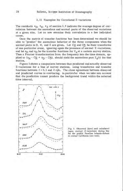
Figure 5 shows a comparison between thus predicted and actually observed<br />
Z -variations for a line of survey stations, using transforms and transfer<br />
functions between f ::: D. 5 and 2 cph. The close agreement between observed<br />
and predicted curves is convincing, in particular when we take into account<br />
that the prediction cannot produce the background trend within the selected<br />
time interval.<br />
Fig. 5. Observed (dots) and calculated<br />
(open circles) Z-variations during bay<br />
for the profile Farallon Islands-Auburn<br />
in central California (see text).


