Schmucker-Weidelt Lecture Notes, Aarhus, 1975 - MTNet

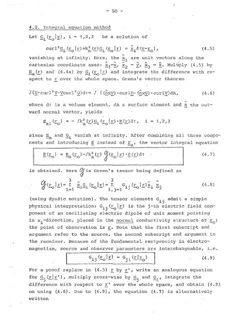
4.2. In3ral - --- equation method
Let -1 G.(r --a [r), -- i = 1,2,3 be a solution of
cur12c. .-I (r --0 lr)+k2 - n (r)G. - --I (r --0 Ir)
,.
A
- = zi6(g-%), (4.5)
vanishing at infinity. Here, the x. are unit vectors along the
A h -l h A A A
cartesian coordinate axes: x =x, x =
-1 - -2 1, z3 = - 2. 14u'iul&31y (4.5) by
E (r) and (4.4a) by G.
-a - (r I?:) and integrate the difference with re-
-1 -0 -
spect to - r over the whole space. Green's vector theorem
where d-r i.s a volume element, dA a surface element and - 1 the out-
ward normal vector, yields
since and G vanish at infinity. After combining all three compo--
-i
nents and introducing - E instead of E , the vector integral equation
-a
1 -gtg)d~ (4.7)
--
is obtained. Here is Green's tensor being defined as
wj(rJ
% --O
3 3 A h
A
t(r Ir)= C x.G. (r [r)= Z G.. (r .Ir)x: x.
- -1-1 -0 - ir j=1
13 -0 -- -1 -3
i= I
(using dyadic notation). The tensor elements G.. admit a simple
= 7
physical interpretation: Gij (r _o [r) - is the j-th electric field coin-
ponent of an oscillating electric di-pole of unit moment pointlng
in x.-direction, placed in the normal conductivity structure at &;
1 --
the point of observation is - r. Note that the first subscript and
argument refer to the source, the second subscript and argument to
the receiver. Because of the fundamental reci.p~:ocity in electro-
mag~~etl.sm, source and observer parameters axe interchangeable, i.e.
For a proof replace in (4.5) - r by - r', write an analogous equation
for G.(rlrl), multiply cross-wise by G and Gi, integrate the
-3 - - - j -
difference wit11 respect to - r' over the whole space, and obtain (4.9)
on using (4 .G) . Due to (4.9) , the equation (4.7) is alternatj.vely
written