Schmucker-Weidelt Lecture Notes, Aarhus, 1975 - MTNet
Schmucker-Weidelt Lecture Notes, Aarhus, 1975 - MTNet Schmucker-Weidelt Lecture Notes, Aarhus, 1975 - MTNet
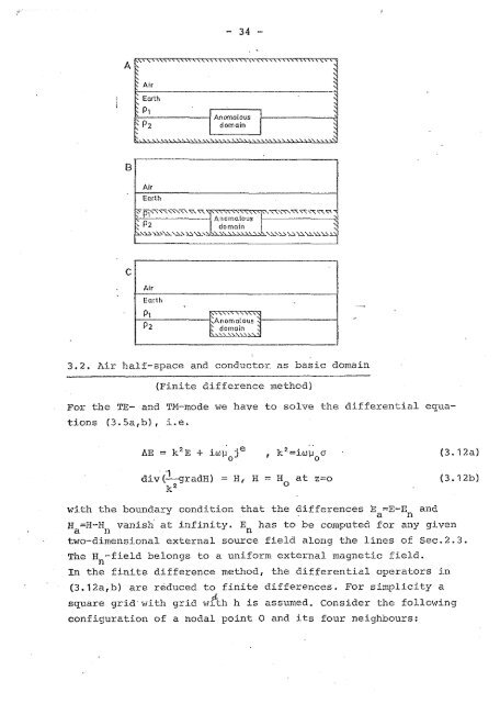
assuming that the TM magnetic source field j.s due to a uniforrn sheet current at height z = -h, h > 0. T1lj.s assun~ptj-on, however, is immaterial for the following. In the sequel all field quantities are split into a normal and anoinalous part, denoted by the subscripts "nu and "a" , respectivel-y. The normal part refers to a one-dimensional conductivity structure. Let u(y,zl = un(z) + U,(Y,Z) (3.7) H(y,z) = Hn(z) + Ha(y,z) E and H are defined as solutions of the equations n n (3.3b) e AEn = k2 E + j (3.10a) n 11 d l d -(- - 1-1 ) = H z > Or H (0) = dz ,?2 dz n n ' - n vanishing for z + m. In virtue of (3.5a,b), (3.9arb), and (3.103,b) Ea and H satisfy a 1 d 1. 1 dIln div (- gradH ) = H a - - - , z > 0 k a k * k2 dz - n If the anomalous domain is of fin2te extent, E has to vanish uni- a forinly at infinity. Under the same condition Ha has to vanish uni- formly in the lower half-space. At z=o H is zero. a If the anomalous domain is of infi.nite extent in horizontal direc- tion, we can demand only that Ear H +O for z + m. a For a numerical solution of (3.11 a) the following three clioices of a basic dornain are possible (boundaries hatched). In approach A, (3.11 a) is solved by Finite differences subject to the boundary condition Ea=O or better subject to an inpedance boundary collclition (below). In approach B (3.11a) is solved by finite differences only in the anomal.ous slab. At the ho~izontal boundaries boundary conditions involicity the normal structure above and below the slab are applied. I approach C (3.11~~) is re- duced to an integral equation over the anon~alous domain. These approaches will now be discussed in details.
i I Earth Anomalous domain 3.2. Air half-space and conductor. as basic domain (Finite difference method) For the TE- and TM-mode we have to solve the differential equa- tions (3.Sa,b), i.e. with the boundary condltion that the differences E =E-E and a n Ha=H-HI> vanish' at infinity. E has to be computed for any given n two-dimensional external source field al.ong the lines of Sec.2.3. The H -field belongs to a uniform external magnetic field. n In the finite difference method, the differential operators in (3.12a,b) are reduced to finite differences. For simplicity a d square grid.with grid ~11th h is assumed. Consider the following configuration of a nodal point 0 and its four neighbours:
- Page 1 and 2: Electromagnetic Induction in the Ea
- Page 3 and 4: 6.2. Generalized matrix inversion 6
- Page 5 and 6: A1~Lernativel.y p = 30. m, where T
- Page 7 and 8: The e1ectrica:L effect - of the cha
- Page 9 and 10: The vari.ables x,y, and t which do
- Page 11 and 12: - d IufM12 > 0 . dz - - On the othe
- Page 13 and 14: a) TM-mode From (2.251, (2.26); (2.
- Page 15 and 16: with " the abbreviation + - 1 - ? =
- Page 17 and 18: 2n -i~cr cos (8-$1 -iKrcU J e ~B=J
- Page 19 and 20: In the 1irnl.t a -+ o, I +- m, M =
- Page 21 and 22: -- 2.5. Definition -- of the transf
- Page 23 and 24: we arrive at - v The same appl-ies
- Page 25 and 26: ) Computation of ---- C for a laxez
- Page 27 and 28: The approximate interpretation of C
- Page 29 and 30: I ~ispersi-on relations I Dispersio
- Page 31 and 32: where L is a positively oriented cl
- Page 33 and 34: 1 2 3 4 CPD 1 2 3 4 CPD - g) Depend
- Page 35: The TE-mode has no vertical electri
- Page 39 and 40: Hence, the conductivity is to be av
- Page 41 and 42: The RHS i.s a closed line integral
- Page 43 and 44: 4. Having determined B;, the coeffi
- Page 45 and 46: 3.4. Anomalous region as basic doma
- Page 47 and 48: - 6 and 6= can be so adjusted that
- Page 49 and 50: From the generalized Green's theore
- Page 51 and 52: and y can again be so adjusted that
- Page 53 and 54: 4.2. In3ral - --- equation method L
- Page 55 and 56: The element GZx is needed for all z
- Page 57 and 58: With this knowledge of the behaviou
- Page 59 and 60: After having determined Qzr VJ,; @,
- Page 61 and 62: 4.3. The surface inteyral approach
- Page 63 and 64: F At the vertical boundaries the co
- Page 65 and 66: The four equations A A A A H = i sg
- Page 68 and 69: 6. Approaches to the inverse proble
- Page 70 and 71: to minimize the quantity a s = 12 /
- Page 72 and 73: It remains to show a way to minimiz
- Page 74 and 75: Agai-n, from a finite erroneous dat
- Page 76 and 77: Here lJ - is a N x P matrix contain
- Page 78 and 79: small eigenvalues. The parameter ve
- Page 80 and 81: Then - 77 - A(E2 - E ) = iwu U (E -
- Page 82 and 83: whence 2k d -2k d where a = CA:(A;)
- Page 84 and 85: . 7. Basic concepts of geomagnetic
i<br />
I Earth<br />
Anomalous<br />
domain<br />
3.2. Air half-space and conductor. as basic domain<br />
(Finite difference method)<br />
For the TE- and TM-mode we have to solve the differential equa-<br />
tions (3.Sa,b), i.e.<br />
with the boundary condltion that the differences E =E-E and<br />
a n<br />
Ha=H-HI> vanish' at infinity. E has to be computed for any given<br />
n<br />
two-dimensional external source field al.ong the lines of Sec.2.3.<br />
The H -field belongs to a uniform external magnetic field.<br />
n<br />
In the finite difference method, the differential operators in<br />
(3.12a,b) are reduced to finite differences. For simplicity a<br />
d<br />
square grid.with grid ~11th h is assumed. Consider the following<br />
configuration of a nodal point 0 and its four neighbours:


