Schmucker-Weidelt Lecture Notes, Aarhus, 1975 - MTNet

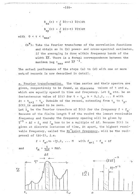
with 0 < T < 'rmax.
R (T) = / Z(+-t) Z(t)dt
Z z T
R (T) = / Z(+-t) YCt)dt
ZY T
x
(b ): Take the Fourier transforms of the correlation functions
and obtain as in (b) power- and cross-spectral estimates,
if the averaging is done within frequency bands of the
width m. There is a formal correspondence between the
-- -1.
maximum lag and Af .
The actual performance of the steps (a) to (d) with one or more
setsof records is now described in detail.
-- a. Fourier transformation. - The time series and their spectra are
given, respectively to be found, at discrete values of t and w,
which are equally spaced in time and frequency. Let Z e-tc. be an
n
.instantenuous value of ZCt) for t = tn, n = 0,1,2, . . . N with
At = tntl - t . Outside of the record, extending from t to t
n o N
Z(t) is assumed to be zero.
-
Let Z be the Fourier transform of Z(t) for the frequency f = f .
n1 IT1
Because of the finite length T of the rec6rd the lowest resolvable
frequency and thereby the frequency spacing w i l l be given by
T-I = Af = f and f has to be a multiple of Af. Because Z(t) is
1 m
gj-ven at discrete instances of -time, A t apart, the hi.ghest resol-
-,
vable frequency, called the Ny quist frequenz, w i l l be the reci-
procal of (At-2), i.e.
and
- I
fH - - = MAf
2At