Marine electromagnetic induction studies - Marine EM Laboratory

MARINE ELECTROMAGNETIC INDUCTION STUDIES 

S. C. CONSTABLE 

IGPP, Scripps Institution of Oceanography, La Jolla, CA 92093, U.S.A. 

Abstract. In reviewing seafloor induction studies conducted over the last seven years, we observe a 

decline in single-station magnetotelluric (MT) experiments in favour of large, multinational, array 

experiments with a strong oceanographic component. However, better instrumentation, processing 

techniques and interpretational tools are improving the quality of MT experiments in spite of the 

physical limitations of the band limited seafloor environment, and oceanographic array deployments are 

allowing geomagnetic depth sounding studies to be conducted. Oceanographic objectives are met by the 

sensitivity of the horizontal electric field to vertically averaged motional currents, providing the same 

information, at much greater reliability and much lower cost, as an array of continuously operating 

current meter moorings. 

The seafloor controlled source method has now become, if not routine, at least viable. Prior to 1982, 

only one seafloor controlled source experiment has been conducted; now at least three groups are 

involved in the experimental aspects of this field. The horizontal dipole-dipole configuration is favoured, 

although a variant of the magnetometric resistivity method utilising a vertical electric transmitter has 

been developed and deployed. By exploiting the characteristics of the seafloor environment, source 

receiver spacings unimaginable on land can be achieved; on a recent deployment dipole spacings of 

90 km were used with a clear 24 Hz signal transmitted through the seafloor. This, and prior experiments, 

show that the oceanic upper mantle is characteristically very resistive, 10all m at least. This resistive 

zone is becoming apparent from other experiments as well, such as studies of the MT response in coastal 

areas on land. 

Mid-ocean ridge environments are likely to be the target of many future electromagnetic studies. By 

taking available laboratory data on mineral, melt and water conductivity we predict to first order the 

kinds of structures the EM method will help us explore. 

1. Introduction 

This review is intended to cover the period since Law's (1983) report on marine 

electromagnetic research, and so the emphasis will be on papers published or 

presented since about 1982. Reviews from before 1982 include those by Cox (1980), 

Filloux (1979), and Fonarev (1982). A more recent review emphasising exploration 

applications is presented by Chave et al. (1990). 

Since 1982 there has been a continued and steady interest in the use of 

magnetotelluric (MT) and geomagnetic depth soundings (GDS) on the seafloor. 

The areas of controlled source and oceanographic use of EM methods, however, 

have seen significant development and expansion. When Law's review was pub- 

lished only one controlled source experiment has been carried out, but now there 

are at least three groups working in this area, and most of the recent large projects 

have a major, if not predominant, component of oceanography, although by their 

very size and nature they must be multi-disciplinary in their objectives. 

The largest project, EMSLAB, resulted in the deployment of 118 instruments in 

1985 and involved a very large group of workers (there are 35 co-authors compris- 

ing The EMSLAB Group, 1988) from six countries. GDS and MT sites covered the 

US states of Oregon and Washington (spilling over into adjacent states and 

Surveys in Geophysics 11: 303-327, 1990. 

9 1990 Kluwer Academic Publishers. Printed in the Netherlands.

304 S.C. CONSTABLE 

Canada) and the seafloor exposure of the Juan de Fuca plate. The main objective 

of this exercise was the delineation of the subducting slab, but oceanography 

and regional geology also motivated the work. The experiment employed mostly 

existing equipment, but the collection of such a large data set has supported and 

encouraged improvements in response function estimation and forward and inverse 

modelling. 

In an effort to obtain detailed structure over the ridge in the EMSLAB area, a 

group of Japanese, Canadians and Australians have deployed 12 instruments 

(yielding 11 magnetometer and 2 E-field sensors) over a small area of the Juan de 

Fuca Ridge (unpublished EMRIDGE deployment cruise report, 1988). These 

instruments were recovered in November, 1988. 

The Tasman project (TPSME) was a joint US/Australian deployment of seafloor 

pressure/MT equipment, across the Tasman Sea between SE Australia and New 

Zealand, for four months in 1983/1984. A landward extension of the traverse (on 

the Australian side) was made using Gough-Reitzel GDS instruments. 

The 1986/1987 BEMPEX (Barotopic ElectroMagnetic and Pressure EXperi- 

ment) study in the North Pacific, in which a total of 41 electric field, pressure and 

magnetic recorders were deployed over a region 1000 km square (Luther et al., 

1987; Chave et al., 1989) is an ambitious project with primarily oceanographic 

goals. This was the longest deployment of these instruments. 

The following sections of this review introduce the marine electromagnetic 

environment, and then consider the areas of geomagnetic and magnetotelluric 

sounding, controlled source methods, and oceanographic studies. Each of these 

sections has a brief introduction followed by a review of recent activity. Finally, the 

use of EM methods in the study of mid-ocean ridges is considered as a means of 

predicting future progress in an area of rapidly expanding research. 

2. The Marine Electromagnetic Environment 

For those more familiar with electromagnetic experiments conducted on, or over, 

the land, the marine environment is a world turned upside-down. Experiments must 

be carried out within a relatively good conductor, the sea, often for the purpose of 

studying the less conductive material of the seafloor below. This conductive 

environment may be advantageous in several ways, however. Movement of seawa- 

ter through the Earth's magnetic field produces an electric field. While this motion 

constitutes a noise source for M.T. at periods longer than an hour (Chave and 

Filloux, 1984), measurement of the electric field can be used to infer large-scale 

water transport. On the deep ocean floor the large conductance of the overlying sea 

severely attenuates short period electromagnetic variations originating in the 

ionosphere. The magnetic field is attenuated more rapidly in frequency than the 

electric field because it is much more sensitive to the resistive seafloor (Chave 

et al., 1990), but by 0.1 Hz both fields are reduced to 0.1% of their surface values. 

This results in an extremely quiet environment for controlled source experiments.

MARINE E.M. 305 

Controlled source studies also benefit from the absence of an air wave; propagation 

at high frequencies (or short times) is solely through the seafloor, which is usually 

the primary region of interest. 

All marine electrical methods benefit from the ease with which contact may be 

made with the environment. Potential electrode noise is lower than experienced on 

land, as temperature, salinity and contact resistance are all nearly constant. Water 

choppers (Filloux, 1987) may be used to reduce low frequency electrode noise 

(below about 0.01 Hz) even further. Controlled source experiments may use trans- 

mission currents of up to 100 A in electric dipoles because a low impedance contact 

to seawater is so easily made. Both electric receivers and electric transmitters may 

be flown through the water, or dragged across the seabed, while making continuous 

electrical contact. 

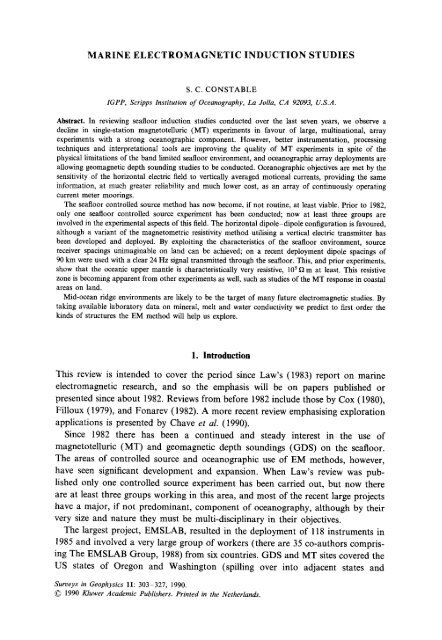
Figure 1 presents a resistivity-depth profile of the oceanic seafloor, based on 

borehole logging and soundings by controlled source and M.T. methods. These 

experiments will be discussed later in this review, but the figure presents an 

instructive summary of seafloor resistivity. 

Seawater resistivity is about 0.3 Qm throughout most of the ocean, although it is 

as low as half this value in warmer, surface waters. In the oceanic crust, electrical 

conductivity is largely controlled by the presence of pore fluids (predominantly 

E 

10 5 

10 4. 

10 3 

.~ 10 2 

re" 

101 

10 0 

@ 

rll 

.> 

0 0 

0 

I 

I 

I 

I 

I 

,, o 

" 

r~ 

.,P 

o 0 

~ m 

m,.j 

10-1 I I I I I i I I I I lill I I 

10-1 10 0 

.7_.0 

u~ 

.~'5 

8~ 

I i i i Ii 

101 

Depth below seafloor, km 

l 

O 

~ 

~, i...: i 

"o .i 

0 ~"" i 

i i i i i i iii I 

10 2 

Fig. 1. Seafloor resistivity as a function of depth, based on data from large scale borehole resistivity 

and interpretations of controlled source and MT soundings. The lithospheric ages are 6.2, 25 and 

30 My respectively. 

~

306 s.c. CONSTABLE 

seawater, but also magma in the ridge areas), varying both with the size and 

connectedness of the fluid passages and with temperature. Saltwater conductivity as 

a function of temperature and pressure has been measured by Quist and Marshall 

(1968). Near-surface, water saturated sediments have high conductivities approach- 

ing that of seawater. Pillow lava resistivities are about 10 tim, while the underlying 

intrusives are less porous and about 1000 g)m. At the Moho porosity drops again, 

and the upper mantle is thought to be very dry, less than 0.1% water, and very 

resistive, 105 f~m or more. 

The mineral conductivity of cool, dry silicates is very low, but increases exponen- 

tially with temperature. The upper mantle is probably composed of a composite of 

olivine and pyroxene with only minor amounts of other minerals. Olivine is the 

dominant mineral both in terms of volume fraction and conductivity, and so has 

attracted considerable attention in laboratory studies of physical properties. The 

most reproducible data have been obtained from single crystal measurements rather 

than those on whole rocks, and Duba et al. (1974) and Schock et al. (1989) report 

conductivities for olivine crystals of mantle composition. Following the lead of 

Shankland and Waft (1977), it became popular to increase the conductivity 

estimated from single crystal studies by a factor of ten to allow for the influence of 

minor minerals and impurities. However, recent work by Constable and Duba 

(1990) indicates that single crystal conductivity may provide a good analogue for 

rock conductivity. These laboratory studies in combination with seafloor sounding 

experiments suggest that upper mantle resistivity between about 30 and 100 km 

drops three orders of magnitude as temperature increases from below 850 ~ to 

around 1400 ~ 

A minimum in resistivity at depths of 100-200 km is generally observed using 

M.T. sounding. This high conductivity zone is usually interpreted as being associ- 

ated with partial melting at the base of the lithosphere. The conductive zone is also 

seen beneath continents, and marks the point at which oceanic and continental 

mantle conductivity structures are indistinguishable. Beneath the conductive zone, 

mantle resistivity appears to rise to about 100 I)m. 

3.1. INTRODUCTION 

3. Geomagnetic Depth Sounding and Magnetotelluric Studies 

Geomagnetic depth sounding (GDS) refers to the deployment of a line or array of 

magnetometers to observe the spatial behaviour of the vector magnetic field as a 

function of frequency. In its simplest form, the vertical field is considered the 

response to the exciting field, which is predominantly horizontal at sharp conductiv- 

ity boundaries such as between the air and land or sea. In an Earth devoid of lateral 

variations in conductivity, there is no vertical field response to a horizontal field, 

and so the method is excellent at detecting and mapping 2D and 3D structure. 

Depth resolution is poor, however, and there are numerous cases in the literature

MARINE E,M. 307 

where current being chaneUed through shallow conduction paths has been inter- 

preted as deeper conductive structure. 

In magnetotelluric (MT) sounding, the horizontal electric field is measured as 

well as the magnetic field. Like the vertical field in GDS, the electric field can be 

considered the response to the exciting horizontal magnetic field, except that now 

there is a response from a laterally uniform Earth. The E/B response as a function 

of frequency may be interpreted to give vertical (1D) conductivity structure, and, if 

an array of stations is available, 2D or 3D structure. 

On the seafloor both methods suffer from the filtering of the external field by the 

ocean at periods on the order of 100 s or shorter and contamination of the magnetic 

field by water motion, beginning with internal waves at periods of about 1 hour and 

extending into longer periods with tides and ocean currents. As a result, MT 

response functions are limited to 2 or 3 decades of frequency. However, as may be 

seen from the example in Figure 1, the MT method samples seafloor conductivity 

at a depth unattainable using other techniques. 

3.2. RECENT ACTIVITY 

Law (1983) predicted that ring-shaped cores in fluxgate sensors would be used to 

improve the sensitivity of seafloor magnetometers. Many groups are indeed in- 

stalling such sensors, and Segawa et al. (1982, 1986) describe such a device. Using 

the data from this test deployment, Yukutake et al. (1983) report preliminary 

results for three MT stations across the Japan Trench, modelling depths of a little 

over 100 km for the conductive upper mantle layer under 125 My old crust. 

Koizumi et al. (1989) deployed a proton precession magnetometer alongside the 

fluxgate instrument in order to establish the drift characteristics of the fluxgate. The 

difference between the total fields from each instrument shows a rapid drift of over 

40 nT during the first four days followed by a more gentle drift of 10 nT over the 

remaining 75 days. The authors consider all the drift to originate within the fluxgate 

device. 

Ferguson et al. (1985) present another preliminary interpretation, this time for 

the Tasman experiment. Models are presented, but the response function for the 

station under consideration exhibited a strong, frequency independent anisotropy. 

Analysis of further stations (Lilley et al., 1989) shows that this behaviour is typical, 

and it is likely that current channelling, or at least the effect of 2D structure, in the 

restricted water of the Tasman Sea is affecting the response functions. The investi- 

gators are currently examining this possibility with the use of thin-sheet modelling. 

The largest seafloor MT experiment to date has been part of the even larger 

EMSLAB project (The EMSLAB Group, 1988; see also the special issue of J. 

Geophys. Res. 94, No B10). Thirty-nine of the EMSLAB instruments were deployed 

on the seafloor between the Washington/Oregon (U.S.A.) coast and the spreading 

zentre at the Juan de Fuca Ridge. It will be some time before this large mass of 

information is fully analysed, but the magnetotelluric data and qualitative interpre- 

tations are presented by Wannamaker et al. (1989a). A model fitting one traverse


on land (the 'Lincoln Line') and five of the seafloor sites is presented by The 

EMSLAB Group (1988) and Wannamaker et al. (1989b), in which a conductive, 

subducting slab is featured. Filloux et al. (1989) discuss the objectives of the 

seafloor part of the experiment and depict Parkinson vectors for the seafloor array. 

The induction vectors show a strong coast effect with little or no distortion 

associated with the ridge. Dosso and Nienaber (1986) and Chen et al. (1989) use an 

analogue model to characterize the magnetic variation pattern expected from a 

subducting Juan de Fuca plate. 

The electrical model presented by Wannamaker et al. (1989b) includes structure 

extending 200 km each side of the coast and to a depth of 400 km. One of the 

principal objectives of the EMSLAB exercise was to study the entire section, from 

oceanic to continental regimes, so the distinction between the marine and non- 

marine aspects of this work becomes somewhat arbitrary. In terms of seafloor 

structure, the model contains a very conductive (1-2 f~m) sedimentary wedge, 

which is about 2 km thick and underlain by a 3000 ~)m lithosphere extending to 

35 km depth. We know from controlled source sounding that this is a simplification 

of the lithospheric structure; it is a little resistive for oceanic crust and is most 

probably too conductive for lithospheric mantle. Oceanic mantle conductivities 

below 35 km in the model are also unusually large; about 2 orders of magnitude 

more conductive than the continental mantle of the same model, and about 1 order 

of magnitude more conductive than the profile presented here in Figure 1 (but 

which has been generated from data over older lithosphere). Partial melting of 7% 

at a depth of 35 km is inferred from the model resistivity of 20 f~m, with melt 

decreasing to zero at a depth of 200 km. This is an unusually large melt fraction; 

most seismologists would be uncomfortable with more than 2-3% (Sato et al., 

1989). Sato et al. also discuss the problems associated with the estimation melt 

fraction from electrical conductivity in this context, citing unknown pressure effects, 

unknown frequency dependence and the unknown effect of grain boundary phases. 

Of these, the unknown effect of pressure on the conductivities of olivine and melt 

is probably the most severe problem as it is difficult to make electrical conductivity 

measurements at high pressure in the laboratory whilst adequately controlling the 

sample environment. One might add to the list of unknowns the oxygen fugacity of 

the mantle, which in turn could be responsible for an order of magnitude uncer- 

tainty in olivine conductivity. The effects of grain boundary phases and frequency 

dependence on olivine conductivity have been demonstrated by Constable and 

Duba (1990) to be minor, at least for the dunite samples they studied. 

Although partial melt may be invoked to explain the resistivity to 200 km depths, 

the EMSLAB model resistivity of 1 ~m between 200 and 400 km presents a 

problem for even the authors to interpret. In view of these generally high conductiv- 

ities, one is concerned that there exists a breakdown in the assumptions of 

two-dimensionality when interpreting the seafloor data. The compensation distance 

(discussed below) implied by the 3000 f~m oceanic lithosphere of the model is 

1000 kin, considerably larger than the tectonic plate being studied. The effects of


non-planar source-field morphology and static distortion on the MT data are 

shown to be minimal by Bahr and Filloux (1989), who demonstrate that estimates 

of the first four harmonics of the Sq response are consistent with plane-wave MT 

responses at similar frequencies. 

In order to obtain more detailed information over the Juan de Fuca Ridge than 

was possible during the EMSLAB experiment, the EMRIDGE programme saw the 

deployment of 12 instruments to obtain 11 magnetometer sites and 2 E-field sites 

within the flanks and depression of the ridge (unpublished EMRIDGE cruise 

report, 1988). All of the instruments were recovered in November 1988, and initial 

results again indicate that there is no conductivity signature for the ridge (Hamano 

et al., 1989), implying the absence of a large, continuous magma chamber. Another 

interesting result reported by Hamano et al. (1989) is that useful E-field data may 

be obtained within the MT frequency band without employing water choppers or 

very long antennae. 

The estimation of lithospheric thickness and its probable increase with age has 

been one of the goals of marine MT sounding for some time. After Oldenburg 

(1981) reported a strong correlation between lithospheric thickness and age, further 

work by Oldenburg et al. (1984) showed that although the data demanded different 

structure beneath the different sites, the correlation with age was not as strong as 

previously thought. 

Niblett et al. (1987) operated a MT station on sea ice in the Arctic Ocean for one 

month. During that time the ice sheet moved back and forth over the Alpha Ridge, 

a topographic high on the Arctic seafloor. Apart from the technical difficulty of 

operating MT equipment in subzero temperature, the experiment is novel because 

in many respects it is equivalent to a seafloor sounding, except of course that the 

measurements were made on the sea surface. The problems of contamination by 

water motion and insensitivity to shallow seafloor structure are the same as those 

for seafloor measurements. The results were very sensitive to seafloor topography, 

and 2D modelling of bathymetry accounted for the anisotropy observed in the data. 

It should be noted that seafloor topography up to 300 km from the measurement 

site was considered to influence the data. No lateral structure in seafloor conductiv- 

ity was required, and the data were fit by a 1000 f~m lithosphere underlain by a 

10 f~m mantle at a depth of 85 km. As noted by the authors, this electrical 

asthenosphere is shallow for the inferred age of the seaftoor in this region (100 My). 

Berdichevsky et al. (1984) used 2D finite difference modelling of a horst type 

structure to conclude that seafloor MT and GDA experiments (in contrast to 

observations at the sea surface) are relatively insensitive to such topographic 

irregularities. 

3.3. THE COAST EFFECT 

It was stated above that the GDS method is particulary sensitive to lateral 

variations in conductivity. The largest variation of this kind is, of course, the 

junction between land and sea, or coast, and indeed the shorelines of the world


produce a marked distortion of the magnetic field at periods of about an hour. The 

distortion is most easily seen in the vertical field, which is of comparable magnitude 

to the horizontal field at the coast and extends inland for many hundreds of 

kilometres. Kendall and Quinney (1983), Singer et al. (1985) and Winch (1989) 

consider the theory of modelling induction in the world ocean. 

Neumann and Hermance (1985) deployed magnetometers at 9 sites perpendicular 

to the Pacific coast in Oregon, U.S.A., and observed a coast effect that was too 

large to be explained by the ocean alone. They concluded that currents induced in 

a thick sedimentary wedge on the continental shelf were required to satisfy the data. 

Kellett et al. (1988a) presented three Parkinson vectors, from part of a larger 

experiment, to demonstrate that the coast effect off SE Australia was largest at the 

middle of the continental slope, as one would expect. Kellett et al. (1988b) present 

Parkinson vectors for an observatory in New Zealand at periods of 200-10 000 s. 

In a modelling study of the coast effect, Fischer and Weaver (1986) examined the 

ability to detect lateral variations in lithospheric conductivity in the presence of the 

strong ocean response. They note that MT methods do not perform very well in 

these circumstances, but that GDS experiments are well suited to the detection of 

lateral conductivity changes, and, in principle, could discriminate lateral litho- 

spheric structure in spite of the strong oceanic response. However, they show that 

the presence of even 100 km of 250 m deep water over the continental shelf prevents 

this discrimination, even when seafloor measurements on the shelf are included. 

Similar modelling was used in a study supported by DeLaurier et al. (1983) to 

interpret 3 seafloor and 2 land magnetometer stations on and off Vanvouver Is., 

Canada. They produce a model featuring a sedimentary wedge and a downward 

dipping conductive slab. Although much of this model is generated by the workers 

preconceptions of the structure, in a later MT analysis of three land stations, Kurtz 

et al. (1986) clearly observe a conductive feature at a depth of about 20km, 

associated with the down-going slab and coincident with a strong seismic reflector. 

This study must be considered the first unambiguous detection of a subducting slab 

using EM methods. 

In a review of Australian conductivity studies, Constable (1990) compiled coast 

effect data for Australia, reproduced here as Figure 2, and noted that the distinction 

between shield regions and younger regimes is not marked, as has been commonly 

proposed. The data are fit reasonably well by a model of Cox et aL (1971) in which 

an ocean of realistic thickness and conductivity is embedded in an infinitely resistive 

lithosphere. The lithosphere is terminated by a conductor at a depth between 240 

and 420 km. The conclusion is that without data beyond the continental shelf there 

is no sensitivity to continental resistivity in this type of experiment. 

It is encouraging to see coast effect studies being supported by quantitative 

modelling, although the non-uniqueness of EM interpretation is a persistent prob- 

lem and the modelling has to rely heavily on structure presumed a priori. Such 

studies have a great advantage in that the predominant feature, the ocean, is 

of known shape and conductivity. Indeed, by utilising analogue modelling the

n- 

b4 

d 

0 

f- 

s 

1.2 0 

0 

\ 

1.0 l\\\ 

0.8 

0.4 

F-- 

X 

O.6 \~ \ 

0.2 

0.0 0 


Australian Coast Effect 

\ 

>**,. 

0 ~ ~ 

Shield 

o Non-shield 

o Transition 

*o000 --*---- 

Oo ,. 

-~o o * 

I I I 

1 O0 200 300 400 

Kilometres from Continental Shelf 

Fig. 2. Compilation of Australian coast effect data from Constable (1990), categorized according to 

geological regime. While the coast effect for shield areas is generally larger than for non-shield areas, 

there is some overlap. The broken lines are models of Cox et al. (1971) with conductors at depths of 240 

(lower curve) and 420 kin. 

response of arbitrarily complex coastal boundaries can be obtained (Herbert et al., 

1983; Chan et al., 1983; Dosso et al., 1985; Hu et al., 1986; Dosso et al., 1986). 

None of the coast effect studies have incorporated the very resistive oceanic 

lithosphere, and one of the most interesting goals of future work will be to examine 

the r61e of continental margins in the leakage of current past this layer. 


4. Controlled Source Methods 

The use of a controlled EM source to study the seafloor has at last come of age. 

There are groups at Cambridge University (U.K.), Toronto University/Pacific 

Geoscience Centre (Canada), and Scripps Institution of Oceanography (U.S.A.) all 

active in this area. The importance of this method lies in the ability to fill the gap 

between deep boreholes a kilometre or two deep and MT sounding, which on the 

deep seafloor is not sensitive to structure shallower than about 50 km. The gap is 

filled by generating at the seafloor the high frequency source field that is removed 

from the natural spectrum by the overlying water, that is at frequencies of 1 Hz plus 

or minus a few decades. In addition to the necessity of providing a high frequency


signal, there are three elements which make seafloor controlled source EM a very 

attractive method: 

Firstly, the absence of a natural signal at the frequencies of operation combined 

with an isothermal and isosaline environment for the receiver electrodes results 

in a very low noise level for electric field receivers; as low as 10-24V 2 m -2 Hz 

above 1 Hz for a 1 km antenna (Webb et al., 1985). Magnetic noise is also lower 

than on land, but magnetometers are vulnerable to motion caused by water currents 

and lack the resolution afforded by E-field receivers employing long antennae. As 

a consequence, magnetic receivers have only been used for relatively shallow 

sounding. 

Secondly, since the seawater absorbs controlled source signals as effectively as 

ionospheric signals of similar frequency, receivers sufficiently far from the source 

never detect energy which has propagated through the seawater. Instead the 

measured signals must travel through the more resistive seafloor, and since the 

seafloor is usually of interest, this is a great advantage. In contrast, on land the 

primary signal propagating through the resistive atmosphere is much larger than 

the signal through the earth. Viewed in terms of time domain sounding, on the 

ocean bottom the signal at early time is sensitive to seafloor conductivity and at late 

times is a measure of seawater conductivity. On land, the early time signal has 

propagated through the atmosphere. 

Thirdly, electrical contact is easily made with seawater, allowing large transmitter 

currents on the order of 100 A and allowing both E-field sources and receivers to 

be dragged through the water during operation. 

We may quantify the comparison between magnetic and electric receivers for 

controlled source sounding. The noise level for the E-field receiver reported by 

Webb et al. (1985) corresponds to a controlled source signal of about 10-is V m- 

per unit dipole moment after typical source strength (2 x l04 Am for a horizontal 

electric dipole) and stacking time (30 rain) are taken into account. As illustrated by 

the models of Chave and Cox (1982), this corresponds to a magnetic field on the 

order of 10 -12 nT, which may be converted to an instrument noise level of 

10-12 nT2/Hz. Noise estimates for seafloor magnetometers in the relevant frequency 

band are difficult to find in the literature, but Wolfgram et al. (1986) report a 

resolution of 10 -3 nT after stacking, which corresponds to 10 -7 nT/Am 2 for the 

source dipole assumed above. From this value it may be concluded that the effective 

range for a horizontal E-field transmitter/B-field receiver combination would be 

about 5 km at 1 Hz. The E-field receivers, on the other hand, are capable of 

measuring the signal to ranges of many tens of kilometers. This having been said, 

it may be noted that below 1 Hz the seafloor E-field spectrum rises more rapidly 

than the magnetic spectrum, and that magnetometers do not suffer from the 1If 

noise which is unavoidable using electrodes until frequencies are low enough for 

water choppers to be practicable. It may be that for controlled source experiments 

in the 10-100 s period range, which might be required for a relatively conductive 

target, magnetometers may be useful in deep controlled source soundings.



There have been several controlled source system geometries deployed in the 

marine environment. The Scripps work has concentrated on the use of seafloor 

horizontal electric dipoles for both the source and receivers, with a fully inductive 

AC signal being broadcast from the transmitter dipole. This geometry is also used 

by the Cambridge group. 

The Toronto/PGC approach has been a variation on the magnetometric resistiv- 

ity method of Edwards (1974), and is described by Edwards, Law and DeLaurier 

(1981). A vertical electric bipole is suspended from a ship to the seafloor; the 

receivers are magnetometers measuring the azimuthal magnetic field generated 

either by an essentially DC current flow in the transmitter or a transmission at 

frequencies high enough to induce secondary currents in the seafloor. 

After the initial successful, but limited, experiment in 1980 by Young and Cox 

(1981) the Scripps group developed the forward modelling theory for the seafloor 

1D Earth (Chave and Cox, 1982; Chave, 1983a) and a more sensitive receiver 

(Webb et al., 1985). In 1984 an experiment was conducted over 25 My old 

seafloor in the northeastern Pacific in which source-receiver spacings of 60 km 

were achieved (Cox et al., 1986). This experiment showed that the bulk resistivity 

of the crust was about 1000 f~m, in good accordance with borehole measurements 

of Becker et al. (1982), and that the upper mantle resistivity was 105 f~m or 

greater. A second experiment recently extended the maximum spacing to 90 km in 

an older (45 My) area of oceanic crust, and qualitatively supported the earlier 

result, since frequencies as high as 24 Hz were again detected at the longest range. 

Such a low conductivity for the upper mantle is a little surprising, but reasonable 

for a model in which the mantle is swept free of volatiles during the formation of 

crust at mid-ocean ridges and then cooled away from the ridges, with very little 

water circulation from the crust into the mantle. 

The vertical electric bipole method has been called MOSES by Edwards et al. 

(1985). The theory for the method is contained in Edwards et al. (1981) and 

Edwards et al. (1984). It is essentially a DC method, generating apparent resistiv- 

ity curves similar to those of resistivity soundings, but Edwards et al. showed that 

if the frequency is made high enough to cause induction in the seafloor, the 

coefficient of anisotropy as well as the average resistivity can be obtained. The 

first experiment using this method was carried out in 640 m of water in Bute Inlet, 

British Columbia, Canada (Edwards et al., 1985). Source-receiver separations up 

to 2000 m were achieved, and a geologically reasonable model of 560 m of 1.9 tim 

of sediment underlain by relatively resistive basement was produced to fit the 

data. 

The second MOSES deployment was a novel experiment near a polymetallic 

sulphide deposit on the Juan de Fuca ridge. Rather than suspending the bipole 

from a ship, a short (100 m) bipole was floated above a seafloor transmitter unit. 

A second seafloor unit was moved to ranges of 30 and 85 m by the submersible


Alvin before other experimental priorities halted the exercise. The data yield 

half-space resistivities of 13 and 20 f~m; in excellent agreement with established 

values for seafloor basalt. It is unfortunate that this experiment could not be 

completed and data collected over the sulphide deposit. 

In what may be regarded as a related experiment, Francis (1985) deployed a 

short (50 m) Wenner resistivity array from a submersible over a sulphide deposit on 

the East Pacific Rise. Resistivities of around 10 f~m for the pillow basalts and as 

low as 0.17 f~m for the sulphide deposit were recorded. Although the experiment 

was extremely simple, these represent the only in situ conductivity measurements of 

seafloor sulphides, and indicate what a useful tool resistivity mapping will be if 

these deposits are to be exploited. 

Having suspended a transmitter from a ship and floated a second from within a 

hydrothermal vent field, it was clear that the next exercise for the Toronto/PGC 

group would be to suspend one from a hole drilled through an ice sheet. This was 

done through ice covering 18 m of water in the Beaufort Sea, in order to map the 

electrically resistive permafrost zone which lies beneath the unfrozen seafloor 

sediments (Edwards et al., 1988). Transmitter-receiver separations of 20-200 m 

were obtained. The data did indeed show evidence of a buried zone at a depth of 

15 m or so with a resistivity an order of magnitude greater than the sediments. An 

attempt was made to study anisotropy by operating at a second, higher (39 Hz) 

frequency, but the researchers were thwarted by noise. 

The Toronto school has been prolific in the generation of background theory for 

various aspects of underwater controlled source EM sounding, including the 

response to transient systems and extension to simple 2D models (Edwards and 

Chave, 1986; Edwards and Cheesman, 1987; Cheesman et al., 1987; Edwards, 

1988a, b; Everett and Edwards, 1989). Most of this theory is directed to a 

completely new area of marine research; that of exploring the continental shelves 

and mid-ocean ridges for natural resources using EM methods. Although early 

attempts have been made using DC methods and a recent dipole-dipole IP system 

was used in search of seafloor mineral sand deposits (Wynn, 1988) both Toronto/ 

PGC and Scripps have recently tested inductive systems, using different geometries. 

The electric dipole-dipole system that works so well in deep water can be modified 

to operate in shallow water in search of shallower targets by increasing the 

frequency of operation to hundreds of hertz (Constable et al., 1986). A magnetic 

dipole-dipole system working in the time domain was operated by Cheesman et al. 

(1988). 


5. Oceanographic Studies 

There has been an increased usage of electromagnetic instruments for oceano- 

graphic purposes. Measurement of the seafloor horizontal electric field gives a 

measure of (orthogonal) horizontal water motion, based on the simple principle


that motion of velocity v through a magnetic field B produces an electric field 

E = v x B. One of the great advantages of this method is that it is mainly sensitive 

to the barotropic (depth independent) component of water flow. Traditional 

oceanographic techniques must employ current meters distributed throughout the 

ocean depth to separate the barotropic and baroclinic components. Recent treat- 

ments of the theory of oceanographic induction are given by Chave and Cox, 

(1983), Chave (1983b) and Chave and Filloux (1984), and Filloux (1987) presents 

a good overview of the method and describes some of the instrumentation involved. 

There are two basic types of motional induction experiments which have been 

performed. In the first type the voltage across a submarine cable is recorded. Under 

favourable circumstances the voltage is a measure of the total water transport 

above the cable. Often the cable spans a channel through which the seawater is 

constrained to flow. If the seafloor is fiat and there are no lateral variations in 

seabed conductivity, the potential across the cable is a linear integral of the water 

motion. That is, the voltage is proportional to the total water transport regardless 

of the spatial distribution of water flow. However, if the seafloor is not fiat, or the 

seabottom conductivity varies laterally, the integral is not linear, and the voltage 

across the cable will-vary if the distribution of water flow varies, even if the total 

transport stays the same. Thus meandering of a water current can corrupt the cable 

voltages as a measure of transport, and is responsible for several failed experiments. 

However, Sanford (1982) demonstrated that measurements of voltage across a 

cable spanning the Florida Straits were consistent with known total water transport 

and seasonal variation, probably because of little lateral motion in the pattern of 

water currents. 

The second type of experiment utilises seafloor electric field recorders, in which 

the voltage is measured across antennae of only a few metres span, effectively giving 

a point measurement of the electric field rather than the integral along a cable. The 

electric field is proportional to the barotropic flow above the instrument, with a 

lateral resolution comparable to the water depth. By deploying an array of seafloor 

recorders, the spatial as well as temporal variations in water transport may be 

monitored. One of the earliest demonstrations of the viability of electric field on the 

deep seafloor as a measure of water transport was made by Cox et al. (1980). 

In both the above methods, the electric field is reduced if significant return 

currents flow through a conductive seafloor. This need not affect the viability of the 

method if the seafloor conductivity is 1D, as the electric field or voltage for a 

resistive seafloor (sometimes called the 'open circuit' voltage) is simply scaled by a 

constant less than or equal to one. The usual practice is to estimate this constant by 

making measurements of water velocity using current meters operated simulta- 

neously with the electrical measurements. 


Larsen and Sanford (1985) estimated water transport of the Florida Current using 

both velocity profiling and potentials measured across a submarine cable. The


agreement between the methods is excellent, and the nearly 2 y of continuous 

electric field data demonstrate that temporal variations in water transport can be 

studied. Such continuous observations would be almost impossible using conven- 

tional profiling. Baines and Bell (1987) attempted to interpret voltages measured 

across the Tasman Sea between Australia and New Zealand, but found no 

systematic variation with transport. The data series was correlated with sea level in 

Sydney, Australia, and is probably mainly sensitive to local currents associated with 

eddies near the Australian end of the cable. 

The motional fields recorded by the EMSLAB experiment are presented by 

Chave et al. (1989). It is shown that the magnetic fields are mainly ionospheric in 

origin for periods below 10 days, but that the electric fields are contaminated (from 

a GDS and MT point of view) by oceanographic signals beyond periods of 2-4 

days. One of the interesting features reported is a southward propagating wave 

attached to the topography of the Juan de Fuca Ridge. 

Oceanographic aspects of the Tasman project are the subject of papers by 

Mulhearn et al. (1986), Bindoff et al. (1986), and Lilley et al. (1986, 1989). In 

particular, they document the seafloor response of a warm-core ring generated by 

the southward-flowing eastern Australian current. 

Early results from the BEMPEX experiment in the North Pacific (personal 

communication with Chave and Luther) indicate that there is negligible electric 

current leaking into seafloor, as predicted by the controlled source observations of 

the crust and upper mantle. A resistive seafloor is desirable on two counts. The 

lateral resolution of an ocean bottom measurement will be improved, and the 

calibration of the experiment with data from current meter moorings become less 

critical. This latter point can be very important when one considers how notoriously 

unreliable current meters are at measuring water motions which are small but not 

necessarily atypical or of insignificant contribution to total transport. However, an 

interesting reversal of the situation occurs when one considers cable measurements, 

which monitor an integral of the electric field. Spain and Sanford (1987) show that 

a large but uniform seafloor conductivity can lessen the detrimental effects of an 

irregular seabed on cable measurements, making it desirable to have a very 

conductive seafloor if the water currents meander in an irregular channel. 

In an unusual application of motional E-field studies, Korotayev et al. (1986) 

estimated water velocities associated with spring water flow from a fracture in the 

Black Sea, by towing a 1500 m electric bipole through the water. In another Black 

Sea study, Korotayev et al. (1985) used the leakage of motionally induced currents 

to estimate the conductivity-thickness product of the seafloor sediments, as well as 

collecting enough magnetic field data to compute an MT response for the area. 

We have only considered the case where the water moves past the sensor. If the 

electric field sensor also moves within the Earth's magnetic field, this motion is also 

the cause of an electric field. Webb and Cox (1982) showed how horizontal electric 

field antennae could detect seismic waves in the frequency range 0.05 to 1 Hz, and 

papers by Webb and Cox (1984) and Webb and Constable (1986) presented data to


support this method. In this frequency band the technique has an advantage over 

accelerometers in that the antenna is better coupled to the seafloor, and unlike 

measurements of pressure the E-field method is sensitive to horizontal motion of the 

seafloor. 

6. Discussion 

6.1. THE RESISTIVE LITHOSPHERIC MANTLE 

The high resistance of mature lithosphere determined from controlled source studies 

has wide implications for seafloor experiments. In order for currents induced in the 

ocean to be able to leak through the resistive region into the conductive mantle 

below, a horizontal scale or compensation distance of L = ~ is required (Cox, 

1980), where S is the longitudinal conductance of the ocean and T is the transverse 

resistance of the lithosphere. From controlled source studies T = 2.5 x 109 tam 2, 

yielding 6000 km for the compensation distance. Singer et al. (1985) used a similar 

value for integrated lithospheric resistance (7 x 109 f~m 2) in their model of global 

induction and concluded that leakage through the lithosphere did occur, and that 

currents induced in the world ocean could go under, rather than around, continents. 

They did observe, however, that compensation distances of 4-5000km were 

required. In a recent paper, Mackie et al. (1988) modelled the transverse resistance 

of the north-eastern Pacific oceanic crust-mantle to be 1 x 109 ~)m 2 from long period 

MT sounding on the adjacent land. This is in excellent agreement with the controlled 

source experiment, and also serves to illustrate the dangers of ignoring oceanic 

induction when analysing coastal MT data. Another estimate of the compensation 

distance was made by Lilley et al. (1989) from a plot of the anisotropy of seafloor 

MT sites as a function of distance from the SE Australian coast. Their data are fit 

very well by a compensation length of 400 km, but this implies a T of only 

2 x 10 7 ~m 2, 2 orders of magnitude smaller than observed in the other experiments. 

However, in the region of their experiment there is only about 800 km of oceanic 

seafloor between Australia and the continental crust of the Lord Howe Rise (and 

even this narrows to the north), and so the seafloor geometry is not ideal for a 

determination of this type. 

For an MT experiment to be interpretable using the 1D approximation, electrical 

structure must be 1D over the compensation scale, or charge will build up on the 

ocean boundaries (the coastlines), reducing the electric field perpendicular to the 

coast. The result will be anisotropic sounding curves even when the seafloor is 

otherwise one-dimensional, with apparent resistivities being too low for the compo- 

nent derived using the E-field perpendicular to the coast. This imposes severe 

restrictions if scales of thousands of kilometres are involved. Motional induction 

studies, however, benefit from the fact that little leakage of induced currents into the 

lithosphere is occurring, and so measurements of the electric field accurately reflect 

horizontal water motion. This is evident in the early results of the BEMPEX 

experiment.


The horizontal scales of the controlled source experiments were only 60-100 km, 

and it is reasonable to suppose the current may leak into the conductive astheno- 

sphere through paths at ridges, continental margins, fracture zones or transform 

faults. However, the study of Mackie et al. (1988) is responsive to a larger region, 

and in particular suggests that no great leakage is occuring at the continental 

margin. It should also be noted that the transverse resistance of the lithosphere is 

probably a function of temperature, and therefore age, of the upper mantle. 

Controlled source soundings have been on 25 My and 45 My old seafloor, but the 

EMSLAB site, for example, is much younger (0-10 My). 

6.2. THE ELECTROMAGNETIC STUDY OF MID-OCEAN RIDGES 

There is a growing interest world wide in the study of mid-ocean ridge systems. To 

understand how ridges behave is to understand how 60% of the Earth's lithosphere 

is generated. Although many of the geophysical studies conducted in the past have 

concentrated on the various seismic techniques, and this trend will undoubtably 

extend into the future, electromagnetic methods have a great advantage in their 

sensitivity to the physical properties under consideration; namely temperature and 

fluid content. Changes which produce only subtle variations in acoustic velocities 

generate orders of magnitude changes in electrical conductivity. 

At the mid-ocean spreading centres upwelling mantle partially melts as a result of 

pressure relief, and this melt then migrates and solidifies to create new oceanic 

crust. Little is known about the mechanisms by which the melt moves from the 

region of melting to crustal depths and then differentiates to form the cumulates, 

dikes, and pillow basalts which make up the crust. Many geometries have at some 

time or other been proposed for the crustal magma chamber which is assumed to 

form, at least at rapid spreading rates and possibly intermittently. Although some 

proportion of melt is required to produce the cumulates we see in ophiolite 

analogues, no one knows if the hypothesised chamber is fully or partially molten. 

Detrick et aL (1987) present a picture of the east Pacific rise (EPR) between 

about 9 ~ and 14 ~ N, based on seismic imaging, in which a liquid upper surface of 

an axial magma chamber is a nearly continuous feature, about 2 km below the 

seafloor and with a width of 2-3 km. The walls and floor of the chamber cannot be 

resolved, but the Moho may be traced to within a few kilometers of the ridge axis, 

suggesting that the width of a magma chamber at this depth (about 6 km) is no 

more than 4-6 km. Expanding spread profiles suggest that only a narrow (about 

1 km) section of the upper surface of the chamber has the unusually low velocities 

associated with mostly molten rock (Harding et al., 1990), but that low velocities on 

the flanks are suggestive of a wider region of hot, mostly solid, rock. Thus we have 

a picture of a narrow (both laterally and vertically) melt accumulation at the top of 

what may be a larger volume of partially molten, or merely hot, material. 

The top of the liquid magma chamber might thus be between 30% melt at a 

temperature of 1185 ~ (Sleep, 1978) and 100% melt at a temperature of 1270 ~ or 

so. The resistivity of tholeiitic melt under these conditions is between 0.5 f~m


(1200 ~ and 0.25 f~m (1300 ~ (Waft and Weill, 1975; Tyburczy and Waft, 1983). 

The dependence of conductivity on melt fraction is less clearly defined. Taking the 

mathematical model presented by Shankland and Waif (1977) which assumes melt 

connectivity, we modify the above figure to get about 2f~m for a 30% melt in the 

magma chamber. Thus we see that the resistivity of the magma chamber is likely to 

vary over one order of magnitude as the melt fraction varies from 30 to 100%. 

Some models for the spreading center have demanded hydrothermal circulation 

through the crust to cool the lower sides of the magma chamber. The results of 

Becker et al. (1982) and Cox et al. (1986) show that older, cooler crust has a 

resistivity of around 1000 f~m between about 1 and 6 km deep, indicating a porosity 

of 1% or so. It is probable that crust close to the ridge axis, thermally cracked and 

with pores not yet plugged with alteration minerals, will have greater porosities. 

However, one notes with interest that Caress (1989) presents a seismic tomography 

model for the EPR at 13~ which features anomalously fast velocities for the 

upper 500 m of the crust within a kilometre or two of the axis. This suggests that 

immediately above the magma chamber cooling has not yet produced significant 

cracking, or that cracking is quickly plugged by intrusives. If this is indeed the case, 

this low porosity cap will be evident in controlled source soundings. The potential 

for electromagnetic experiments to address the question of porosity variations is 

improved by saltwater conductivity not being as sensitive to temperature variations 

one might expect. The average temperature of the older crust is about 100 ~ 

Seawater has a maximum conductivity at 300-400 ~ which is only double its 

conductivity at 100 ~ (Quist and Marshall, 1968), so water saturated rock with 

porosity similar to that of the old crust, no matter how hot, should not have a 

resistivity much above 500 f~m (assuming, of course, that it does not become hot 

enough for silicate conduction to dominate). 

Extrusive lavas at the very top of the crust are much less resistive, about 10 D.m 

based on the measurements of Francis (1985) and Becker et al. (1982) as well as 

reasonable estimates at porosity (10-15%) and fluid conductivity. Primitive magma 

feeding any magma chamber is probably not much hotter than the magma 

chamber. The different chemistry of this material will not alter its conductivity 

significantly from that of the tholeiitic melt described above (Waft and Weill, 1975). 

Estimates of bulk conductivity for this region obtained from EM studies are 

admirably suited to discriminate between porous flow models and models of dike or 

conduit injection. For the 2% porosities required by the porous flow models, 

Shankland and Waif's model predicts resistivities of 10 to 20 f~m. Olivine resistivity 

at 1300 ~ is at least 100 f~m, so assuming an episodic injection model, or a system 

of cracks which are not interconnected all the time, this higher resistivity would be 

observed. 

Both controlled source and GDS methods may prove useful in discriminating 

between the various tectono-physical models. The controlled source experiment of 

Cox et al. (1986) on older crust was sensitive to mantle conductivity to at least 

20 km depth. As argued above and also indicated by the Young and Cox (1981)


experiment, the conductivity of the crust near the ridge is not likely to be more than 

a few times more conductive than at older sites, so similar penetration depths are 

possible a few 10's of kilometres from the ridge. GDS experiments are admirably 

suited to mapping lateral variations in conductivity, and although they have no 

resolution in the resistive crust and upper mantle, conductive melt regions make an 

ideal target. GDS and MT studies to date, however, have failed to detect any 

continuous conductive zone along a ridge (Filloux and Tarits, 1986; Filloux et al., 

1989; Hamano et al. 1989). 

It could be very important for the purposes of a ridge GDS or MT study to know 

where the resistive upper mantle layer terminates. Currents channelled along the 

surface of this layer and then penetrating the mantle at a ridge may have a marked 

effect on the electromagnetic signature; the anomalous electric field perpendicular to 

the EPR seen by Filloux and Tarits (1986) might be such an effect. 

Of as much interest as the fluids in the ridge system is the off-axis temperature 

distribution, both in the crust and the upper mantle. Our knowledge of the 

conductivity of saltwater and olivine as a function of temperature should allow 

suitably placed controlled source soundings to give an indication of the rate of 

cooling within the lower crust/upper mantle, which in turn will indicate the extent 

of hydrothermal circulation. 

In June of 1989 a joint Cambridge/Scripps expedition to the EPR at 13~ 

collected controlled source data for several days, using a specially constructed (by 

Cambridge) transmitting antenna designed to be neutrally bouyant and flown a few 

tens of metres above the rugged seafloor. At the time of writing the data had only 

been examined to the extent that the operation of the transmitter and seven 

receivers was verified, but a few simple 1D models illustrate the sensitivity of the 

dipole-dipole method to hypothetical ridge structures. The basic model we have 

taken consists of an ocean 2.5 km deep, a layer of extrusives on the seafloor which 

is 500 m thick and has a resistivity of 10 f~m, beneath this a crustal layer of 

intrusives and gabbros which is 5.5 km thick and 250 f~m, and finally a mantle 

region of 100 tim (olivine at 1300 ~ 

Figure 3(a) shows the response of this basic model (circles) at a source-receiver 

spacing of 40 kin, and a second model in which the mantle is replaced with partially 

molten material of 10f~m resistivity (diamonds). The broken line represents an 

estimated noise level for the Scripps controlled source system as deployed in the 

1984 experiment. (The solid lines are merely smooth curves joining the actual 

computations of the electric field denoted by the symbols). Although 40 km is the 

largest range at which the signal is above the noise, this long range presents an 

interesting picture of EM propagation. At a frequency of 0.25 Hz we observe that 

the model with the more conductive mantle actually results in a larger signal. This 

is a consequence of the resistive, crustal, layer acting in a manner which may be 

loosely called a waveguide. At certain frequencies the efficiency of this waveguide is 

improved by the greater conductivity contrast presented by the more conductive 

mantle, and so a larger signal is seen. At frequencies lower than 0.25 Hz we see the


effect of energy being lost more readily to the partially molten mantle material of 

the second model, and so depressing the observed signal. 

Figure 3(b) presents the situation closer to the ridge where the lower crust may 

still be above 1000 ~ and so below about 100 f~m. A source-receiver spacing of 

20 km is considered. The curves show the response of such an isotherm at a depth 

of 2.5 km (circles) and 4.5 km (diamonds). Finally, Figure 3(c) shows a sounding 

10--11 

~E 10-15 

~ I0-16 

L~ 10-17 

Ld 

10-18 

A: Mantle model, ronge = 40 kin. 

i i iiiii i i i i iiiii i i I i iiiii I I I~'~1~1~11 

10-2 10-1 100 101 

B: Crustal isotherm model, range = 20 km. 

10-14 ~ 0 

~ 10-15 

Q) 

ts 

,,, 10-16 

> 

k~ 

I.d 

10-12 

I IIII I I I 

10-1 100 101 

C: Magma chamber model, range = 5 km. 

I I r II I I I I I I III I I L I I I III I 

10-1 100 101 

Frequency, Hz 

Fig. 3. Controlled source electric field response over 3 pairs of contrasting models: (A) partially molten 

(diamonds) and merely hot (circles) upper mantle, (B) a crustal I000 ~ isotherm at depths of 2.5 km 

(circles) and 4.5 km (diamonds), and (C) a crustal magma chamber which is fully (diamonds) or 30% 

(circles) molten. The broken line in (A) represents a typical noise level for the Scripps sounding 

equipment. The notch in the noise at 0.1 Hz is a permanent part of the natural spectrum.


immediately over the ridge axis with the source-receiver spacing reduced to 5 km. 

The two models purport to show a magma chamber at a depth of 2 km containing 

partially molten (2 f~m, circles) and fully molten (0.3 tim, diamonds) rock. 

Although the 1D models considered above provide an indication of the sensitivity 

of the controlled source method to ridge structures, they are clearly inadequate for 

quantitative modelling of what is obviously not a 1D structure. 

Ridges are good candidates for 2D modelling, and indeed one is struck by how 

remarkably 2D they are, with hundreds of kilometres between significant offsets. 

While 2D MT modelling is becoming commonplace, the difficulty associated with 

controlled source modelling is that the source-field is 3D. However, progress is 

being made, and forward models of ridges in which the approximation that the 

source is 2D have been presented by Everett and Edwards (1989) for time-domain 

sounding and Flosadottir and Cox (1989) for frequency-domain sounding. The 

models of Everett and Edwards show that the maximum response to a crustal 

magma chamber for a time-domain system occurs at delay times of about 1 s. 

6.3. FUTURE PROGRESS 

We are seeing diminishing returns from the deployment of single-station MT sites 

on the seafloor. There is little prospect of significantly expanding the limited 

frequency band available between long period contamination by oceanic effects and 

short period cutoff due to screening of the source field, and so resolution is 

necessarily limited to a narrow depth range in the upper mantle. On the other hand, 

the expanding use of long period E-field instruments for the study of oceanography 

is likely to support the continued deployment of seafloor EM arrays, from which we 

shall continue to extract MT and GDS data. Magnetic measurements are much 

easier to collect than electric field data, which to date have required either 

sophisticated water choppers or long antennae, but GDS offers possibilities in the 

discrimination of lateral changes in structure across features like ridges; thus one 

expects to see expansion in this area. Already there is a lot of international 

cooperation, reflecting the fact that once a ship is available for an experiment, more 

instruments can be deployed than are usually available to one institution. There will 

be reduced motivation for one facility to maintain a large suite of instruments if this 

continues. 

Controlled source experiments are more difficult (and so more costly and with a 

higher instrument loss) than GDS and MT studies, but offer the chance to study the 

first 50 km or so which is invisible to MT sounding. Now that ground has been 

broken in this area, we will see an expanding use of this method. Although the oil 

and mining industries are currently depressed world-wide, there is academic activity 

in developing EM exploration techniques for the seafloor which might well blossom 

during the next rejuvenation of the industry, whenever that may be. 

A scientific/political emphasis on exploring mid-ocean ridge environments has 

improved the prospects for a vigorous programme of EM experiments in the 

intermediate future, and an EM component is being considered important by many


of the groups coordinating ridge studies. However, these are not easy areas to work 

in and represent challenges to the various disciplines; problems include conductive 

material (controlled source method), dimensionality problems (MT), and topo- 

graphical inhospitability (all methods). We must be cautious not to promise more 

than we can achieve. 

Acknowledgements 

This review was presented at the ninth workshop on electromagnetic induction, held 

at Dagomys, U.S.S.R, in September 1988. The author thanks the program commit- 

tee for the invitation to present the work, and also C. deGroot-Hedlin, who 

delivered the paper in his absence. Most of the author's marine experience has been 

obtained during collaborative work with C. Cox over the last six years, an 

association which has always been instructive and occasionally exciting. He would 

like to thank A. Chave for making his controlled source forward modelling 

program available, amd M. Kappus for the translation of Singer et al. (1985). 

Finally, he expresses his appreciation to all those researchers who responded to his 

request for material associated with marine EM. This review was produced while 

working under NSF grant OCE-8719245. 

References 

Bahr, K. and Filloux, J. H.: 1989, 'Local Sq Response Functions from EMSLAB data', J. Geophys. Res. 

94, 14195-14200. 

Baines, P. G. and Bell, R. C.: 1987, 'The Relationship between Ocean Current Transports and Electric 

Potential Differences across the Tasman Sea, Measured Using an Ocean Cable', Deep-Sea Res. 34, 

531-546. 

Becker, K. and 13 others.: 1982, ' In situ Electrical Resistivity and Bulk Porosity of the Oceanic Crust 

Costa Rica Rift', Nature 300, 594-598. 

Berdichevsky, M. N., Zhdanova, O. N., and Yakovlev, A. G.: 1984, 'Anomalous Electromagnetic Fields 

and Electromagnetic Sounding on the Bottom of the Ocean', Geomag. Aeronomy 24, 542-547. 

Bindoff, N. L., Filloux, J. H., Mulhearn, P. J., Lilley, F. E. M., and Ferguson, I. J.: 1986, 'Vertical 

Electric Field Fluctuations at the Floor of the Tasman Abyssal Plain', Deep-Sea Res. 33, 587-600. 

Caress, D. W.: 1989, Some Aspects of the Structure and Evolution of Oceanic Spreading Centers, 

Unpublished Thesis, Univ. Calif., San Diego. 

Chan, E., Dosso, H. W., Law, L. K., Auld, D. R., Nienaber, W.: 1983, 'Electromagnetic Induction in 

the Queen Charlotte Islands Region: Analogue Model and Field Station Results', J. Geomagn. 

Geoelectr. 35, 501-516. 

Chave, A. D.: 1983a, 'Numerical Integration of Related Hankel Transforms by Quadrature and 

Continued Fraction Expansion', Geophysics 48, 1671-1686. 

Chave, A. D.: 1983b, 'On the Theory of Electromagnetic Induction in the Earth by Ocean Currents', J. 

Geophys. Res. 88, 3531-3542. 

Chave, A. D. and Cox, C. S.: 1982, 'Controlled Electromagnetic Sources for Measuring Electrical 

Conductivity Beneath the Oceans, 1, Forward Problem and Model Study', J. Geophys. Res. 87, 

5327-5338. 

Chave, A. D. and Cox, C. S.: 1983, 'Electromagnetic Induction by Ocean Currents and the Conductivity 

of the Oceanic Lithosphere', J. Geomagn. Geoelectr. 35, 491-499. 

Chave, A. D. and Filloux, J. H.: 1984, 'Electromagnetic Induction Fields in the Deep Ocean off 

California: Oceanic and Ionospheric Sources', Geophys. J. R. Astr. Soc. 77, 143-171.


Chave, A. D., Filloux, J. H., Luther, D. S., Law, L. K., and White, A.: 1989, 'Observations of Motional 

Electromagnetic Fields During EMSLAB', J. Geophys. Res. 94, 14153-14166. 

Chave, A. D., Constable, S. C., and Edwards, R. N.: 1990, 'Electrical Exploration Methods for the 

Seafloor', in Nabighian M. N. (ed.), SEG Electromagnetic Methods in Applied Geophysics, (in press). 

Chave, A. D., Filloux, J. H., and Luther, D. S.: 1989, 'Electromagnetic Induction by Ocean Currents: 

BEMPEX', Phys. Earth Planet. Inter. 53, 350-359. 

Cheesman, S. R., Edwards, R. N., and Chave, A. D.: 1987, 'On the Theory of Sea-Floor Conductivity 

Mapping Using Transient Electromagnetic Systems', Geophysics 52, 204-217. 

Cheesman S. J., Edwards, R. N., and Law, L. K.: 1988, 'First Results of a New Short Baseline Sea Floor 

Transient EM System', Presented at the 58th Ann. Int. Mtg., Soc. Explor. Geophys. in Anaheim, 

U.S.A. 

Chen, J., Dosso, H. W., and Nienaber, W.: 1989, 'Laboratory Electromagnetic Model Results for the 

EMSLAB Region', J. Geophys. Res. 94, 14167-14172. 

Constable, S. C.: 1990, 'Electrical Studies of the Australian Lithosphere', in Drummond, B. J. (ed.), The 

Australian Lithosphere, Geol. Soc. Aust. Spee. Pub. (in press). 

Constable, S. C., Cox. C. S., and Chave, A. D.: 1986, 'Offshore Electromagnetic Surveying Techniques', 

Soc Explor. Geophys, 56th Ann. Internat Mtg. Extended Abstracts, pp. 81-82. 

Constable, S. C. and Duba, A.: 1990, 'The Electrical Conductivity of Olivine, a Dunite and the Mantle', 

J. Geophys. Res. (in press). 

Cox, C. S.: 1980, 'Electromagnetic Induction in the Oceans and Inferences on the Constitution of the 

Earth', Geophys. Surv. 4, 137-156. 

Cox, C. S., Filloux, J. H., and Larsen, J.: 1971, 'Electromagnetic Studies of Ocean Currents and 

Electrical Conductivity Below the Ocean Floor', in Maxwell (ed.), The Sea, Vol. 4 Part 1, Wiley, pp. 

637-693. 

Cox, C. S., Filloux, J. H., Gough, D. I., Larsen, J. C., Poehls, K. A., von Herzen, R. P., and Winter, 

R.: 1980, 'Atlantic Lithospheric Sounding', in U. Schmucker, (ed.), Electromagnetic Induction in the 

Earth and Moon, Centr. Acad Publ. Japan, Tokyo and Kluwer Acad. Publ. Dordrecht, pp. 13-32. 

Cox, C. S., Constable, S. C., Chave, A. D., and Webb, S. C.: 1986, 'Controlled Source Electromagnetic 

Sounding of the Oceanic Lithosphere', Nature 320, 52-54. 

DeLaurier, J. M., Auld, D. R., and Law, L. K.: 1983, 'The Geomagnetic Response across the 

Continental Margin off Vancouver Island: Comparison of Results from Numerical Modelling and 

Field Data', J. Geomagn. Geoelectr. 35, 517-528. 

Detrick, R. S., Buhl, P., Vera, E., Mutter, J., Orcutt, J., Madsen, J., and Brocher, T.: 1987, 

'Multi-Channel Seismic Imaging of a Crustal Magma Chamber Along the East Pacific Rise', Nature 

326, 35-41. 

Dosso, H. W., Nienaber, W., and Parkinson, W. D.: 1985, 'An Analogue Model Study of Electromag- 

netic Induction in the Tasmanian Region', Phys. Earth Planet. Inter. 39, 118-133. 

Dosso, H. W., Chart, G. H., and Nienaber, W.: 1986, 'An Analogue Model Study of EM Induction for 

an Island near Bay and Cape Coastlines', Phys. Earth Planet. lnter. 42, 178-183. 

Dosso, H. W. and Nienaber, W.: 1986, 'A Laboratory Electromagnetic Model Study of the Juan de Fuea 

Plate Region', Phys. Earth Planet. lnter. 43, 34-46. 

Duba, A., Heard, H. C., and Schock, R. N.: 1974, 'Electrical Conductivity of Olivine at High Pressure 

and Under Controlled Oxygen Fugacity', J. Geophys. Res. 79, 1667-1673. 

Edwards, R. N.: 1974, 'The Magnetometric Resistivity (MMR) Method and its Application to the 

Mapping of a Fault', Can. J. Earth Sci. 11, 1136-1156. 

Edwards, R. N.: 1988a, 'A Downhole Magnetometric Resistivity Technique for Electrical Sounding 

Beneath a Conductive Surface Layer', Geophysics 53, 528-536. 

Edwards, R. N.: 1988b, 'Two-Dimensional Modeling of a Towed in-Line Electric Dipole-Dipole Sea 

Floor Electromagnetic System: The Optimum Time Delay or Frequency for Target Resolution', 

Geophysics 53, 528-536. 

Edwards, R. N., Law, L. K., DeLaurier, J. N.: 1981, 'On Measuring the Electrical Conductivity of 

the Oceanic Crust by a Modified Magnetometric Resistivity Method', J. Geophys. Res. 86, 11609- 

11615. 

Edwards, R. N., Nobes, D. C., and Grmez-Trevifio, E.: 1984, 'Offshore Electrical Exploration of 

Sedimentary Basins: The Effects of Anisotropy in Horizontally Isotropic, Layered Media', Geophysics 

49, 566-576.


Edwards, R. N., Law, L. K., Wolfgram P. A., Nobes, D. C., Bone, M. N., Trigg, D. F., and DeLaurier, 

J. M.: 1985, 'First Results of the MOSES Experiment: Sea Sediment Conductivity and Thickness 

Determination, Bute Inlet, British Columbia, by Magnetometric Offshore Electrical Sounding', 

Geophysics 50, 153-160. 

Edwards, R. N. and Chave, A. D.: 1986, 'A Transient Electric Dipole-Dipole Method for Mapping the 

Conductivity of the Sea Floor', Geophysics 51, 984-987. 

Edwards, R. N. and Cheesman S. J.: 1987, 'Two-Dimensional Modelling of a Towed Transient Magnetic 

Dipole-Dipole Sea Floor EM System', J. Geophys. 61, 110-121. 

Edwards, R. N., Wolfgram, P. A., and Judge, M. N.: 1988, 'The ICE-MOSES Experiment: Mapping 

Permafrost Zones Electrically Beneath the Beaufort Sea', Mar. Geophys. Res. 9, 265-290. 

EMSLAB Group.: 1988, 'The EMSLAB Electromagnetic Sounding Experiment', EOS 69, 89, 98-99. 

Everett, M. E. and Edwards, R. N.: 1989, 'Electromagnetic Expression of Axial Magma Chambers', 

Geophys. Res. Lett. 16, 1003-1006. 

Ferguson, I. J., Filloux, J. H., Lilley, F. E. M., Bindoff, N. L., and Mulhearn, P. J.: 1985, 'A Seafloor 

Magnetotelluric Sounding in the Tasman Sea', Geophys, Res. Lett. 12, 545-548. 

Filloux, J. H.: 1979, 'Magnetotelluric and Related Electromagnetic Investigations in Geophysics', Rev. 

Geophys. Space Phys. 17, 282-294. 

Filloux, J, H.: 1987, 'Instrumentation and Experimental Methods for Oceanic Studies', in J. A. Jacobs, 

(ed.), Geomagnetism, Academic Press, pp. 143-248. 

Filloux, J. H. and Tarits, P.: 1986, 'Pacific Rise: Electrical Conductivity Anomaly at Ridge Crust and 

Implications on Structure (abstract)', EOS 67, 919. 

Filloux, J. H., Law, L. K., Yukutake, T., Segawa, J., Hamao, Y., Utada, H., White, A., Chave, A., 

Tarits, P., and Green, A. W.: 1989, 'OFFSHORE EMSLAB: Objectives, Experimental Phase and 

Early Results', Phys. Earth Planet. Inter. 53, 422-431. 

Fischer, G. and Weaver, J. T.: 1986, 'Theoretical Investigations of the Ocean-Coast Effect at a Passive 

Continental Margin', Phys. Earth Planet. Inter. 42, 246-254. 

Flosadottir, A. H and Cox, C. S.: 1989, 'Modeling of the Electromagnetic Controlled Source Response 

of Two Dimensional Mid-Ocean Ridge Structures (abstract)', EOS 70, 1074. 

Fonarev, G. A.: 1982, 'Electromagnetic Research in the Ocean', Geophys. Sum 4, 501-508. 

Francis, T. J. G.: 1985, 'Resistivity Measurements of an Ocean Floor Sulphide Mineral Deposit from the 

Submersible Cyana', Marine Geophys. Res. 7, 419-438. 

Hamano, Y., Segawa, J., Law, L. K., White, A., Heinson, G., Utada, H., and Yukutake, Y.: 1989, 'An 

Electromagnetic Sounding Across the Juan de Fuca Ridge (EMRIDGE)', Contributed paper pre- 

sented at 6th assembly of IAGA in Exeter, U.K. 

Harding, A. J., Orcutt, J. A., Kappus, M. E., Vera, E. E., Mutter, J. C., Buhl, P., Detrick, R. S., and 

Brocher, T. M.: 1989, 'Structure of Young Oceanic Crust at 13 ~ N on the East Pacific Rise from 

Expanding Spread Profiles', J. Geophys. Res. 94, 12163-12196. 

Herbert, D., Dosso, H. W., and Nienaber, W.: 1983, 'Analogue Model Study of Electromagnetic 

Induction in the Newfoundland Region', Phys. Earth Planet. Inter. 32, 65-84. 

Herbert, D., Wright, J. A., Dosso, H. W., and Nienaber, W.: 1983, 'Comparison of Analogue Model and 

Field Station Results for the Newfoundland Region', J. Geomagn. Geoelectr. 35, 673-682. 

Hu, W. B., Dosso, H. W., and Nienaber, W.: 1984, 'Analogue-Model Magnetic Field Responses of an 

Ocean Channel, an Island and a Seamount in the Hainan Island Region', J. Geophys. 55, 222-227. 

Kellett, R. L., White, A., Ferguson, I. J., and Lilley, F. E. M.: 1988a, Geomagnetic Fluctuation 

Anomalies Across the Southeast Australian Coast', Explor. Geophys. 19, 294-297. 

Kellett, R. L., I. J. Ferguson, and Lilley, F. E. M.: 1988b, 'Magnetic Field Fluctuations at the Eyrewell 

Observatory, Christchurch, New Zealand', New Zealand J. Geol. Geophys. 31, 87-93. 

Kendall, P. C. and Quinney, D. A.: 1983, 'Induction in the Oceans', Geophys. J. R. Astr. Soc. 74, 

239 -255. 

Koizumi, K., Segawa, J., Toh, H., Oubina Carretero, J. L., and Tanaka, Y.: 1989, 'Simultaneous 

Magnetic Measurements and their Comparison at the Sea Floor Using a Fluxgate Vector Magnetome- 

ter and a Proton Scalar Magnetometer', J. Geomagn. Geoelectr. 41, 491-506. 

Korotayev, S. M., Trofimov, I. L., Zhdanov, M. S., Shabelyanskiy, S. V., Lapitskiy, A. I., Abroamov, 

Yu. M., and Gaydash, S. P.: 1985, 'Electromagnetic Investigations in the Southwest Portion of the 

Black Sea', Geomag. Aeronomy 25, 228-232.


Korotayev, S. M., Kutkin, V. V., and Lapitsky, A. I.: 1986, 'Investigation of the Filtration Anomaly of 

Natural Electric Field in the Western Part of the Black Sea', Ann. Geophys. 4, 639-644. 

Kurtz, R. D., DeLaurier, J. M., and Gupta, J. C.: 1986, 'A Magnetotelluric Sounding Across Vancouver 

Island Sees the Subducting Juan de Fuca Plate', Nature 321, 596-599. 

Larsen, J. C. and Sanford, T. B.: 1985, 'Florida Current Volume Transports from Voltage Measure- 

ments', Science 227, 302-304. 

Law, L. K.: 1983, 'Marine Electromagnetic Research', Geophys. Surv. 6, 123-135. 

Lilley, F. E. M., Filloux, J. H., Bindoff, N. L., Ferguson, I. J., and Mulhearu, P. J.: 1986, 'Baro- 

tropic Flow of a Warm-Core Ring from Seafloor Electric Measurements', J. Geophys. Res. 91, 

979 -984. 

Lilley, F. E. M., Filloux, J. H., Ferguson, I. J., Bindoff, N. L., and Mulhearn, P. J.: 1989, 'The Tasman 

Project of Seafloor Magnetotelluric Exploration: Experiment and Observations', Phys. Earth Planet. 

lnter. 53, 405-421. 

Luther, D. S., Chave, A. D., and Filloux, J. H.: 1987, 'BEMPEX: A Study of Barotropic Ocean Currents 

and Lithospheric Conductivity', EOS 68, 618-619, 628-629. 

Mackie, R. L., Bennett, B. R., and Madden, T. R.: 1988, 'Long-Period Magnetotelluric Measurements 

Near the Central California Coast: A Land-Locked View of the Conductivity Structure Under the 

Pacific Ocean', Geophys J. 95, 181-194. 

Mulhearn, P. J., Filloux, J. H., Lilley, F. E. M., Bindoff, N. L., and Ferguson, I. J.: 1986, 'Abyssal 

Currents During the Formation and Passage of a Warm-Core Ring in the East Australian Current', 

Deep-Sea Res. 33, 1563-1576. 

Neumann, G. A. and Hermance, J. F.: 1985, 'The Geomagnetic Coast Effect in the Pacific Northwest of 

North America', Geophys, Res. Lett. 12, 502-505. 

Niblett, E. R., Kurtz, R. D., and Michaud, C.: 1987, 'Magnetotelluric Measurements over the Alpha 

Ridge', Phys. Earth Planet. lnter. 45, 101-118. 

Oldenburg, D. W.: 1981, 'Conductivity Structure of Oceanic Upper Mantle Beneath the Pacific Plate', 

Geophys. J. R. Astr. Soc. 65, 359-394. 

Oldenburg, D. W., Whittall, K. P., and Parker, R. L.: 1984, 'Inversion of Ocean Bottom Magnetotelluric 

Data Revisisted', J. Geophys. Res. 89, 1829-1833. 

Quist, A. S. and Marshall, W. L.: 1968, 'Electrical Conductances of Aqueous Sodium Chloride Solutions 

from 0 to 800 ~ and at Pressures to 4000 Bars', J. Phys. Chem. 71, 684-703. 

Sanford, T.: 1982, 'Temperature Transport and Motional Induction in the Florida Current', J. Mar. Res. 

40 (suppl), 621-639. 

Sato, H., Sacks, I. S., and Murase, T.: 1989, 'The Use of Laboratory Velocity Data for Estimating 

Temperature and Partial Melt Fraction in the Low-Velocity Zone: Comparison with Heat Flow and 

Electrical Conductivity Studies', J. Geophys. Res. 94, 5689-5704. 

Schock, R. N., Duba, A., and Shankland, T. J.: 1989, 'Electrical Conduction in Olivine', J. Geophys. 

Res. 94, 5829-5839. 

Segawa, J., Yukutake, T., Hamano, Y., Kasuga, T., and Utada, H.: 1982, 'Sea Floor Measurements of 

the Geomagnetic Field Using Newly Developed Ocean Bottom Magnetometers', J. Geomagn. 

Geoelectr. 34, 571-585. 

Segawa, J., Hamano, Y., Yukutake, T., Utada, H., and Tou, H.: 1986, 'A Sea Floor Magnetometer 

Model OBM-S4', J. Geodetic Soc. Japan 32, 248-273. 

Shankland, T. J. and Waft, H. S.: 1977, 'Partial Melting and Electrical Conductivity Anomalies in the 

Upper Mantle', J. Geophys. Res. 82, 5409-5417. 

Singer, B. S., Kuvshinov, A. V., and Fainberg, E. B.: 1985, Electrical Induction in the Spherical Earth, 

Covering the lnhomogeneous Oceans and in Contact with a Stratified Section, Inst. Terrestrial Mag- 

netism, Ionosphere and Radio Wave Propagation, preprint No. 46. 

Sleep, N. H.: 1978, 'Thermal Structure and Kinematics of Mid-Oceanic Ridge Axis, some Complications 

to Basaltic Volcanism', Geophys, Res. Lett. 5, 426-428. 

Spain, P, and Sanford, T. B.: 1987, 'Accurately Monitoring the Florida Current with Motionally 

Induced Voltages', J. Mar. Res. 45, 843-870. 

Tyburczy, J. A. and Waft, H. S.: 1983, 'Electrical Conductivity of Molten Basalt and Andesite to 25 

kilobars Pressure: Geophysical Significance and Implications for Charge Transport and Melt Struc- 

ture', J. Geophys. Res. 88, 2413-2430.


Waft, H, S. and WeiU, D. F.: 1985, 'Electrical Conductivity of Magrnatic Liquids: Effects of Tempera- 

ture, Oxygen Fugaeity and Composition', Earth Planet. Sci. Lett. 28, 254-260. 

Wannamaker, P. E. and 14 others.: 1989a, 'Magnetotelluric Observations across the Juan de Fuca 

Subduction System in the EMSLAB Project', J. Geophys. Res. 94, 14111-14t25. 

Wannamaker, P. E., Booker, J. R., Jones, A. G., Chave, A. D., Filloux, J. H., Waft, H. S., and Law, 

L. K.: 1989b, 'Resistivity Cross Section Through the Juan de Fuca Subduction System and its 

Tectonic Implications', J. Geophys. Res. 94, 14127-14144. 

Webb, S. C. and Cox, C. S.: 1982, 'Electromagnetic Fields Induced at the Seafloor by Rayleigh-Stoneley 

Waves', J. Geophys. Res. 87, 4093-4102. 

Webb, S. C. and Cox, C. S.: 1984, 'Pressure and Electric Fluctuations on the Deep Sea Floor: 

Background Noise for Seismic Detection', Geophys, Res. Lett. 11, 967-970. 

Webb, S. C., Constable, S. C., Cox, C. S., and Deaton, T.: 1985, 'A Seafloor Electric Field Instrument', 

J. Geomagn. Geoelectr. 37, 1115-1130. 

Webb, S. C. and Cox, C, S.: 1986, 'Observations and Modeling of Seafloor Microseisms', J. Geophys. 

Res. 91, 7343-7358. 

Webb, S. C. and Constable, S. C.: 1986, 'Microseism Propagation Between Two Sites on the Deep 

Seafloor', Bull, Seis. Soc. Am. 76, 1433-1445. 

Winch, D. E.: 1989, 'Induction in a Model Ocean', Phys. Earth Planet. Inter. 53, 328-336. 

Wolfgram, P. A., Edwards, R. N., Law, L. K., and Bone, M. N.: 1986, 'Polymetallic Sulphide 

Exploration on the Deep Sea Floor: The Feasibility of the MINI-MOSES Experiment', Geophysics 51, 

1808-1818. 

Wynn, J. C.: 1988, 'Titanium Geophysics: The Application of Induced Polarization to Sea-Floor Mineral 

Exploration', Geophysics 53, 386-401. 

Young, P. D. and Cox, C. S.: 1981, 'Electromagnetic Active Source Sounding near the East Pacific Rise', 

Geophys, Res. Lett. 8, 1043-1046. 

Yukutake, T., Filloux, J. H., Segawa, J., Hamano, Y., and Utada, H.: 1983, 'Preliminary Report on a 

Magnetotelluric Array Study in the Northwest Pacific', J. Geomagn. Geoelectr. 35. 575-587.

Marine electromagnetic induction studies - Marine EM Laboratory

Create successful ePaper yourself

Delete template?

Save as template?