lambert universal variable algorithm - Arabian Journal for Science ...

M.A. Sharaf, A.N. Saad, and M.I. Nouh
where χ is to be considered as a new independent variable — a kind of generalized anomaly. It could be shown
[12] that when χ is used as the independent variable instead of the time t, then the non-linear equations of motion
can be converted into linear, constant coefficients, differential equations.
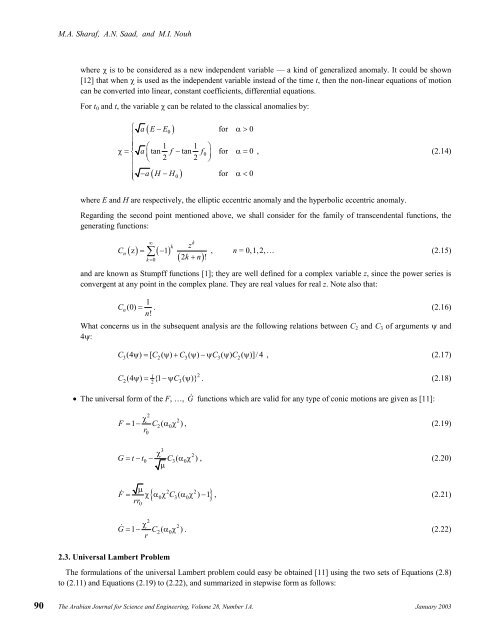
For t0 and t, the variable χ can be related to the classical anomalies by:
( )
⎧ a E−E0for α > 0
⎪
⎪ ⎛ 1 1 ⎞
χ= ⎨ a⎜tan f −tan f0for
α= 0
2 2
⎟
, (2.14)
⎪ ⎝ ⎠
⎪
⎪⎩
−a( H −H0) for α < 0
where E and H are respectively, the elliptic eccentric anomaly and the hyperbolic eccentric anomaly.
Regarding the second point mentioned above, we shall consider for the family of transcendental functions, the
generating functions:
C
n
∞
( z) = ∑ ( −1)
k = 0
k
k
z
, n = 0,1,2,… (2.15)
2 !
( k + n )
and are known as Stumpff functions [1]; they are well defined for a complex variable z, since the power series is
convergent at any point in the complex plane. They are real values for real z. Note also that:
1
Cn(0)
= . (2.16)
n !
What concerns us in the subsequent analysis are the following relations between C2 and C3 of arguments ψ and
4ψ:
C (4 ψ ) = [ C ( ψ ) + C ( ψ) −ψC ( ψ) C ( ψ)]/4
, (2.17)
3 2 3 3 2
1
2 2 3
2
C (4 ψ ) = {1 −ψC ( ψ)}
. (2.18)
• The universal form of the F, …, G functions which are valid for any type of conic motions are given as [11]:
2
χ
2
F = 1 − C2(
α0χ) , (2.19)
r
0
3
χ
2
G = t−t0 − C 3( α0χ) , (2.20)
µ
0
2 2
{ 0 3( 0 ) 1}
F
µ
= χ α χ C α χ −
rr
2.3. Universal Lambert Problem
2
, (2.21)
G
χ
2
= 1 − C2(
α0χ) . (2.22)
r
The formulations of the universal Lambert problem could easy be obtained [11] using the two sets of Equations (2.8)
to (2.11) and Equations (2.19) to (2.22), and summarized in stepwise form as follows:
90 The Arabian Journal for Science and Engineering, Volume 28, Number 1A. January 2003