the development of poiseuille flow of a pseudoplastic fluid

M.A.M. Al Khatib
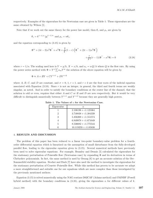
respectively. Examples of the eigenvalues for the Newtonian case are given in Table 1. These eigenvalues are the
same obtained by Wilson [1].
Note that if we work out the same theory for the power law model, then θ◦ and µ◦ are given by
θ◦ = k 1−1/n |y| 1−1/n and µ◦ = nθ◦,
and the equation corresponding to (3.15) is given by
Φ iv +(4r − 2)α 2 Φ ′′
+ α 4 Φ+ 2
(1 − r) Φ
Y ′′′
+(2r− 1)α 2 Φ ′
+ r
(r − 1)(Φ′′ − α
Y 2 2 Φ) = 0 (3.18)
where r =1/n. The scaling used here is Y = y/h, X = x/h, andu◦ = uQ/h where Q is the flow rate. By using
the power series method with Φ = Y σ amY m the solution of the above equation will be given by
Φ ≈ A + BY + CY r+1 + DY r+2
where A, B, C, and D are constant, and σ =0, 1, r+1, and r + 2 are the four roots of the indicial equation
associated with Equation (3.18). Since r is not an integer, in general, the third and fourth terms are weakly
singular, as noted. And in order to satisfy the boundary conditions at the center line of the channel, that the
solution is odd or even, requires that either A and C or B and D are zero respectively. But it would be very
difficult to distinguish numerically between Y r+1 and Y r+2 because they are generally high powers.
4. RESULTS AND DISCUSSION
Table 1. The Values of α for the Newtonian Case.
Eigenvalue α
1 2.106196 + i1.125364
2 3.748838 + i1.384339
3 5.356269 + i1.551574
4 6.949978 + i1.671049
5 8.536682 + i1.775544
6 10.119259 + i1.85838
The problem of this paper has been reduced to a linear two-point boundary-value problem for a fourthorder
differential equation which is linearized on the assumption of small disturbance from the fully-developed
parallel flow, leading to the eigenvalue equation given in (3.15). Several numerical methods have previously
been used to solve eigenvalue equations. For example, Bramley and Dennis [5] calculated the eigenvalues for
the stationary perturbation of Poiseuille flow (Newtonian case) by expanding Φ and its derivatives in terms of
Chebyshev polynomials. In fact, the same method is used by Orszag [6] to get an accurate solution of the Orr–
Sommerfeld stability equation. Stocker and Duck [7] have also used the method to investigate the eigenvalues for
the stationary perturbation of Couette–Poiseuille flow. While this method has proven to be accurate we adopt
a more straightforward and suitable one for our equations which are more complex than those investigated by
the previously mentioned authors.
Equation (3.15) is solved numerically using the NAG routines D02CAF (Adams method) and C02NBF (Powell
hybrid method) with the boundary conditions in (3.16), giving the eigenvalues α for different values of k.
January 2006 The Arabian Journal for Science and Engineering, Volume 31, Number 1A. 107