the development of poiseuille flow of a pseudoplastic fluid
the development of poiseuille flow of a pseudoplastic fluid the development of poiseuille flow of a pseudoplastic fluid
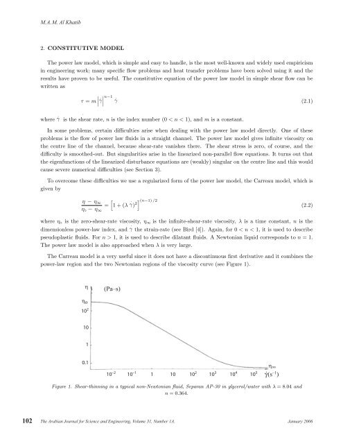
102 M.A.M. Al Khatib 2. CONSTITUTIVE MODEL The power law model, which is simple and easy to handle, is the most well-known and widely used empiricism in engineering work; many specific flow problems and heat transfer problems have been solved using it and the results have proven to be useful. The constitutive equation of the power law model in simple shear flow can be written as τ = m . γ . . n−1 . γ (2.1) where γ is the shear rate, n is the index number (0
3. EQUATIONS OF MOTION M.A.M. Al Khatib We consider a region far downstream from the entrance of a straight channel of width 2h, with the origin in the centre of the channel. The velocity components of the flow in the downstream, x, and transverse, y, directions are u and v respectively. The smoothed-out power law model which is going to be used here, the Carreau Model, is given in 3-dimensional form by Equation (2.2) with · γ= 2eijeij (see Bird [4]). With η∞ = 0 for simplicity, we get where e ∗ ij τ ∗ ij =2η◦ is the strain-rate tensor. 1+(λ · γ) 2(n−1) /2 e ∗ ij By neglecting the inertial effects, the equations of motion in the steady state in the x and y directions are given respectively by 0=− ∂P∗ ∂x + ∂τ∗ xx ∂x + ∂τ∗ xy ∂y , 0=− ∂P∗ ∂y + ∂τ∗ xy ∂x + ∂τ∗ yy ∂y . First we determine the basic parallel flow which is approached far downstream. Here the pressure gradient is uniform and we put − ∂P ∂x = Gr > 0 for convenience. Then from (3.2) we get 0=Gr + ∂τ∗ xy ∂y January 2006 The Arabian Journal for Science and Engineering, Volume 31, Number 1A. 103 (3.1) (3.2) . (3.3) Integrating (3.3) with respect to y using the symmetry condition τ ∗ xy = 0 when y =0weget τ ∗ xy = −Gr y . (3.4) Using Equations (3.1) and (3.4) we get −Gr y = η◦ 1+(λ (u ∗ ◦) ′ ) 2 (n−1) /2 where (u ∗ ◦) ′ = ∂u ∗ ◦/∂y and the subscript ◦ refers to the parallel flow solution. (u ∗ ◦) ′ . (3.5) Now we choose dimensionless variables; we put Y = y/h, X = x/h, P = P ⋆ /Gr h, τij = τ ∗ ij /Grh, and u◦ = η◦u∗ ◦/Grh2 . Then the dimensionless form of the solution is given by the following equations t◦ = −Y, (3.6) −Y = 1+k 2 ( u ′ ◦) 2 (n−1)/2 u ′ ◦ , (3.7) where t◦ and u ′ ◦ are the stress and velocity derivative in the case of parallel flow and k =(λGrh)/η◦. Note that when k is large, (3.7) represents a shear thinning fluid and when k is small, (3.7) represents a Newtonian fluid. Equation (3.7) is solved numerically with the boundary condition u◦ = 0 when Y = −1, giving u ′ ◦ and u◦. Examples of velocity profiles are given in Figures 2, 3, and 4.
- Page 1: THE DEVELOPMENT OF POISEUILLE FLOW
- Page 5 and 6: velocity 0.6 0.5 0.4 0.3 0.2 0.1 0
- Page 7 and 8: M.A.M. Al Khatib respectively. Exam
- Page 9 and 10: Table 4. The Leading Eigenvalue α
102<br />
M.A.M. Al Khatib<br />
2. CONSTITUTIVE MODEL<br />
The power law model, which is simple and easy to handle, is <strong>the</strong> most well-known and widely used empiricism<br />
in engineering work; many specific <strong>flow</strong> problems and heat transfer problems have been solved using it and <strong>the</strong><br />
results have proven to be useful. The constitutive equation <strong>of</strong> <strong>the</strong> power law model in simple shear <strong>flow</strong> can be<br />
written as<br />
<br />
<br />
τ = m . <br />
γ<br />
<br />
.<br />
.<br />
n−1 . γ (2.1)<br />
where γ is <strong>the</strong> shear rate, n is <strong>the</strong> index number (0


