the development of poiseuille flow of a pseudoplastic fluid
the development of poiseuille flow of a pseudoplastic fluid
the development of poiseuille flow of a pseudoplastic fluid

Create successful ePaper yourself
Turn your PDF publications into a flip-book with our unique Google optimized e-Paper software.
THE DEVELOPMENT OF POISEUILLE FLOW OF A<br />
PSEUDOPLASTIC FLUID<br />
M.A.M. Al Khatib<br />
HBCC, King Fahd University <strong>of</strong> Petroleum & Minerals<br />
KFUPM Box 5087, Dhahran, Saudi Arabia<br />
e-mail: alkhatibm@yahoo.com<br />
M.A.M. Al Khatib<br />
1. INTRODUCTION<br />
We consider here <strong>the</strong> two-dimensional steady <strong>flow</strong> <strong>of</strong> a liquid down a semi-infinite straight<br />
channel, a much-studied problem <strong>of</strong> obvious practical and <strong>the</strong>oretical interest. Far from <strong>the</strong><br />
entrance, <strong>the</strong> <strong>flow</strong> is parallel to <strong>the</strong> walls and <strong>the</strong> determination <strong>of</strong> <strong>the</strong> velocity distribution is<br />
a simple matter, whatever <strong>the</strong> constitutive model. We consider here <strong>the</strong> region sufficiently far<br />
downstream that <strong>the</strong> <strong>flow</strong> is almost parallel, so that <strong>the</strong> equations can be linearized about <strong>the</strong><br />
parallel-<strong>flow</strong> solution. We <strong>the</strong>n look for <strong>the</strong> approach to fully-developed <strong>flow</strong> by way <strong>of</strong> decaying<br />
eigenmodes. This was done for <strong>the</strong> Newtonian liquid by Wilson [1]. In that paper both large<br />
and small Reynolds numbers were considered; here we consider only low Reynolds number. This<br />
is reasonable in view <strong>of</strong> <strong>the</strong> generally large viscosity <strong>of</strong> <strong>the</strong> liquids.<br />
Al Khatib and Wilson [2] extended that work to <strong>the</strong> case <strong>of</strong> viscoplastic liquids. Viscoplastic<br />
liquids have a yield stress; little or no motion <strong>of</strong> <strong>the</strong> <strong>fluid</strong> will occur until a critical yield stress<br />
is exceeded. Al Khatib and Wilson expected that <strong>the</strong>re should be two types <strong>of</strong> regions <strong>of</strong> a<br />
viscoplastic liquid in <strong>the</strong> channel; an unyielded region which is at <strong>the</strong> center <strong>of</strong> <strong>the</strong> channel, and<br />
yielded regions which are close to its walls. These regions are separated by <strong>the</strong> yield surface.<br />
For a Bingham <strong>fluid</strong> this natural assumption turns out to be kinematically impossible because<br />
<strong>of</strong> <strong>the</strong> absolute rigidity <strong>of</strong> <strong>the</strong> unyielded region assumed by <strong>the</strong> Bingham model. To overcome<br />
this difficulty, <strong>the</strong>y used <strong>the</strong> smoo<strong>the</strong>d-out form <strong>of</strong> <strong>the</strong> Bingham model; biviscosity model. They<br />
showed that as <strong>the</strong> biviscosity model approaches <strong>the</strong> Bingham model, <strong>the</strong> approach <strong>of</strong> <strong>the</strong> entry<br />
<strong>flow</strong> to <strong>the</strong> fully-developed parallel <strong>flow</strong> becomes infinitely delayed.<br />
This paper extends <strong>the</strong> above work to <strong>the</strong> case <strong>of</strong> Pseudoplastic (shear thinning) liquids.<br />
The viscosity <strong>of</strong> <strong>pseudoplastic</strong> liquids decreases as <strong>the</strong> shear rate increases. Greases, mayonnaise,<br />
many polymers, polymer solutions, and suspensions exhibit this type <strong>of</strong> behavior (see Tanner [3]).<br />
The next section gives more details about <strong>the</strong> power law and Carreau models which are used<br />
to describe <strong>pseudoplastic</strong> liquids.<br />
Key words: power law model, Pseudoplastic <strong>fluid</strong>s, Carreau model, two-point boundary-value problem.<br />
Paper Received 17 January 2004; Revised 8 October 2004; Accepted 26 March 2005.<br />
January 2006 The Arabian Journal for Science and Engineering, Volume 31, Number 1A. 101
102<br />
M.A.M. Al Khatib<br />
2. CONSTITUTIVE MODEL<br />
The power law model, which is simple and easy to handle, is <strong>the</strong> most well-known and widely used empiricism<br />
in engineering work; many specific <strong>flow</strong> problems and heat transfer problems have been solved using it and <strong>the</strong><br />
results have proven to be useful. The constitutive equation <strong>of</strong> <strong>the</strong> power law model in simple shear <strong>flow</strong> can be<br />
written as<br />
<br />
<br />
τ = m . <br />
γ<br />
<br />
.<br />
.<br />
n−1 . γ (2.1)<br />
where γ is <strong>the</strong> shear rate, n is <strong>the</strong> index number (0
3. EQUATIONS OF MOTION<br />
M.A.M. Al Khatib<br />
We consider a region far downstream from <strong>the</strong> entrance <strong>of</strong> a straight channel <strong>of</strong> width 2h, with <strong>the</strong> origin<br />
in <strong>the</strong> centre <strong>of</strong> <strong>the</strong> channel. The velocity components <strong>of</strong> <strong>the</strong> <strong>flow</strong> in <strong>the</strong> downstream, x, and transverse, y,<br />
directions are u and v respectively.<br />
The smoo<strong>the</strong>d-out power law model which is going to be used here, <strong>the</strong> Carreau Model, is given in<br />
3-dimensional form by Equation (2.2) with · γ= 2eijeij (see Bird [4]). With η∞ = 0 for simplicity, we get<br />
where e ∗ ij<br />
τ ∗ ij =2η◦<br />
is <strong>the</strong> strain-rate tensor.<br />
<br />
1+(λ · γ) 2(n−1) /2<br />
e ∗ ij<br />
By neglecting <strong>the</strong> inertial effects, <strong>the</strong> equations <strong>of</strong> motion in <strong>the</strong> steady state in <strong>the</strong> x and y directions are<br />
given respectively by<br />
0=− ∂P∗<br />
∂x + ∂τ∗ xx<br />
∂x + ∂τ∗ xy<br />
∂y ,<br />
0=− ∂P∗<br />
∂y + ∂τ∗ xy<br />
∂x + ∂τ∗ yy<br />
∂y .<br />
First we determine <strong>the</strong> basic parallel <strong>flow</strong> which is approached far downstream. Here <strong>the</strong> pressure gradient is<br />
uniform and we put − ∂P<br />
∂x = Gr > 0 for convenience. Then from (3.2) we get<br />
0=Gr + ∂τ∗ xy<br />
∂y<br />
January 2006 The Arabian Journal for Science and Engineering, Volume 31, Number 1A. 103<br />
(3.1)<br />
(3.2)<br />
. (3.3)<br />
Integrating (3.3) with respect to y using <strong>the</strong> symmetry condition τ ∗ xy = 0 when y =0weget<br />
τ ∗ xy = −Gr y . (3.4)<br />
Using Equations (3.1) and (3.4) we get<br />
−Gr y = η◦<br />
<br />
1+(λ (u ∗ ◦) ′ ) 2 (n−1) /2<br />
where (u ∗ ◦) ′ = ∂u ∗ ◦/∂y and <strong>the</strong> subscript ◦ refers to <strong>the</strong> parallel <strong>flow</strong> solution.<br />
(u ∗ ◦) ′ . (3.5)<br />
Now we choose dimensionless variables; we put Y = y/h, X = x/h, P = P ⋆ /Gr h, τij = τ ∗ ij /Grh, and<br />
u◦ = η◦u∗ ◦/Grh2 . Then <strong>the</strong> dimensionless form <strong>of</strong> <strong>the</strong> solution is given by <strong>the</strong> following equations<br />
t◦ = −Y, (3.6)<br />
−Y =<br />
<br />
1+k 2 ( u ′<br />
◦) 2 (n−1)/2<br />
u ′<br />
◦ , (3.7)<br />
where t◦ and u ′<br />
◦ are <strong>the</strong> stress and velocity derivative in <strong>the</strong> case <strong>of</strong> parallel <strong>flow</strong> and k =(λGrh)/η◦. Note<br />
that when k is large, (3.7) represents a shear thinning <strong>fluid</strong> and when k is small, (3.7) represents a Newtonian<br />
<strong>fluid</strong>. Equation (3.7) is solved numerically with <strong>the</strong> boundary condition u◦ = 0 when Y = −1, giving u ′<br />
◦ and u◦.<br />
Examples <strong>of</strong> velocity pr<strong>of</strong>iles are given in Figures 2, 3, and 4.
104<br />
M.A.M. Al Khatib<br />
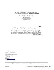
Figure 2. The velocity pr<strong>of</strong>iles <strong>of</strong> <strong>the</strong> Carreau model with k =2and for different values <strong>of</strong> n.<br />
velocity<br />
10<br />
9<br />
8<br />
7<br />
6<br />
5<br />
4<br />
3<br />
2<br />
1<br />
0<br />
0 –0.8 –0.6 –0.4 –0.2 0 0.2 0.4 0.6 0.8 1<br />
V<br />
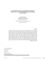
Figure 3. The velocity pr<strong>of</strong>iles <strong>of</strong> <strong>the</strong> Carreau model with k =10and for different values <strong>of</strong> n.<br />
The Arabian Journal for Science and Engineering, Volume 31, Number 1A. January 2006<br />
n=0.3<br />
n=0.5<br />
n=0.8<br />
n=1
velocity<br />
0.6<br />
0.5<br />
0.4<br />
0.3<br />
0.2<br />
0.1<br />
0<br />
-1 -0.8 -0.6 -0.4 -0.2 0<br />
y<br />
0.2 0.4 0.6 0.8 1<br />
M.A.M. Al Khatib<br />
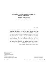
Figure 4. The velocity pr<strong>of</strong>iles <strong>of</strong> <strong>the</strong> Carreau model with k =0.5 and for different values <strong>of</strong> n (curves from top to bottom<br />
are, respectively, n =0.1, 0.2, 0.3, 0.5, 0.8, 1).<br />
The velocity pr<strong>of</strong>iles in Figures 2 and 3 correspond to <strong>the</strong> case k>1. They indicate that <strong>the</strong> velocity gradients<br />
near <strong>the</strong> boundaries diverge as <strong>the</strong> index n tends to 0. In fact, it is easy to prove from Equation (3.7) for k>1<br />
and small n that<br />
|u ′ ◦(±1)| = k 1/n−1 .<br />
On <strong>the</strong> o<strong>the</strong>r hand, this divergence does not exist if k
106<br />
M.A.M. Al Khatib<br />
The constitutive Equation (3.1) becomes, in dimensionless form,<br />
After linearization we find<br />
<br />
τij =2 1+k 2 · γ 2 (n−1) /2<br />
eij. (3.10)<br />
∂u1<br />
τ1 XX =2θ◦<br />
∂X<br />
∂v1<br />
τ1YY =2θ◦<br />
∂Y<br />
τ1 XY = µ◦<br />
∂u1<br />
∂Y<br />
<br />
∂v1<br />
+<br />
∂X<br />
where θ◦ =(1+k 2 u ′ 2<br />
◦ ) (n−1)/2 and µ◦ = θ◦<br />
1+nk 2 u ′ 2<br />
◦<br />
1+k 2 u ′ 2<br />
◦<br />
.<br />
(3.11)<br />
From (3.9) and (3.11) with u1 =ΨY and v1 = −ΨX, where Ψ is <strong>the</strong> stream function, we have<br />
∂2 ∂X∂Y (4θ◦ΨXY<br />
2 ∂ ∂2<br />
)+ −<br />
∂Y 2 ∂X2 <br />
[µ◦(ΨYY − ΨXX)] = 0 (3.12)<br />
and <strong>the</strong> boundary conditions on <strong>the</strong> walls Y = ±1 are<br />
Now let<br />
Ψ(X, ±1) = 0, ΨY (X, ±1) = 0. (3.13)<br />
Ψ=Φ(Y ) exp(−αX) (3.14)<br />
as in Wilson [1]. Substituting (3.14) in (3.12) we get<br />
<br />
2 d<br />
4α<br />
dY<br />
with boundary conditions<br />
θ◦<br />
2<br />
2 dΦ d d Φ<br />
+ − α2 µ◦<br />
dY dY 2 dY 2 − α2 <br />
Φ = 0 (3.15)<br />
Φ(±1) = Φ ′ (±1) = 0 (3.16)<br />
and this determines <strong>the</strong> eigenvalues α. These are complex in general and we are interested in <strong>the</strong> decaying modes<br />
for which Re(α) > 0. Note that when k =0,orn =1weget<br />
θ◦ = µ◦ =1,<br />
and we recover <strong>the</strong> Newtonian case<br />
Φ iv +2α 2 Φ ′′<br />
+ α 4 Φ = 0 (3.17)<br />
studied by Wilson [1]. The eigenvalues satisfy sin 2α = ±2α, with four families <strong>of</strong> roots, one in each quadrant<br />
<strong>of</strong> <strong>the</strong> complex plane. The two signs in sin 2α = ±2α correspond to odd and even solutions to Equation (3.15),<br />
The Arabian Journal for Science and Engineering, Volume 31, Number 1A. January 2006
M.A.M. Al Khatib<br />
respectively. Examples <strong>of</strong> <strong>the</strong> eigenvalues for <strong>the</strong> Newtonian case are given in Table 1. These eigenvalues are <strong>the</strong><br />
same obtained by Wilson [1].<br />
Note that if we work out <strong>the</strong> same <strong>the</strong>ory for <strong>the</strong> power law model, <strong>the</strong>n θ◦ and µ◦ are given by<br />
θ◦ = k 1−1/n |y| 1−1/n and µ◦ = nθ◦,<br />
and <strong>the</strong> equation corresponding to (3.15) is given by<br />
Φ iv +(4r − 2)α 2 Φ ′′<br />
+ α 4 Φ+ 2<br />
<br />
(1 − r) Φ<br />
Y ′′′<br />
+(2r− 1)α 2 Φ ′<br />
+ r<br />
(r − 1)(Φ′′ − α<br />
Y 2 2 Φ) = 0 (3.18)<br />
where r =1/n. The scaling used here is Y = y/h, X = x/h, andu◦ = uQ/h where Q is <strong>the</strong> <strong>flow</strong> rate. By using<br />
<strong>the</strong> power series method with Φ = Y σ amY m <strong>the</strong> solution <strong>of</strong> <strong>the</strong> above equation will be given by<br />
Φ ≈ A + BY + CY r+1 + DY r+2<br />
where A, B, C, and D are constant, and σ =0, 1, r+1, and r + 2 are <strong>the</strong> four roots <strong>of</strong> <strong>the</strong> indicial equation<br />
associated with Equation (3.18). Since r is not an integer, in general, <strong>the</strong> third and fourth terms are weakly<br />
singular, as noted. And in order to satisfy <strong>the</strong> boundary conditions at <strong>the</strong> center line <strong>of</strong> <strong>the</strong> channel, that <strong>the</strong><br />
solution is odd or even, requires that ei<strong>the</strong>r A and C or B and D are zero respectively. But it would be very<br />
difficult to distinguish numerically between Y r+1 and Y r+2 because <strong>the</strong>y are generally high powers.<br />
4. RESULTS AND DISCUSSION<br />
Table 1. The Values <strong>of</strong> α for <strong>the</strong> Newtonian Case.<br />
Eigenvalue α<br />
1 2.106196 + i1.125364<br />
2 3.748838 + i1.384339<br />
3 5.356269 + i1.551574<br />
4 6.949978 + i1.671049<br />
5 8.536682 + i1.775544<br />
6 10.119259 + i1.85838<br />
The problem <strong>of</strong> this paper has been reduced to a linear two-point boundary-value problem for a fourthorder<br />
differential equation which is linearized on <strong>the</strong> assumption <strong>of</strong> small disturbance from <strong>the</strong> fully-developed<br />
parallel <strong>flow</strong>, leading to <strong>the</strong> eigenvalue equation given in (3.15). Several numerical methods have previously<br />
been used to solve eigenvalue equations. For example, Bramley and Dennis [5] calculated <strong>the</strong> eigenvalues for<br />
<strong>the</strong> stationary perturbation <strong>of</strong> Poiseuille <strong>flow</strong> (Newtonian case) by expanding Φ and its derivatives in terms <strong>of</strong><br />
Chebyshev polynomials. In fact, <strong>the</strong> same method is used by Orszag [6] to get an accurate solution <strong>of</strong> <strong>the</strong> Orr–<br />
Sommerfeld stability equation. Stocker and Duck [7] have also used <strong>the</strong> method to investigate <strong>the</strong> eigenvalues for<br />
<strong>the</strong> stationary perturbation <strong>of</strong> Couette–Poiseuille <strong>flow</strong>. While this method has proven to be accurate we adopt<br />
a more straightforward and suitable one for our equations which are more complex than those investigated by<br />
<strong>the</strong> previously mentioned authors.<br />
Equation (3.15) is solved numerically using <strong>the</strong> NAG routines D02CAF (Adams method) and C02NBF (Powell<br />
hybrid method) with <strong>the</strong> boundary conditions in (3.16), giving <strong>the</strong> eigenvalues α for different values <strong>of</strong> k.<br />
January 2006 The Arabian Journal for Science and Engineering, Volume 31, Number 1A. 107
108<br />
M.A.M. Al Khatib<br />
Examples <strong>of</strong> <strong>the</strong> eigenvalues are given in Tables 2, 3, and 4 for <strong>the</strong> same values <strong>of</strong> k used to draw <strong>the</strong> velocity<br />
pr<strong>of</strong>iles in Figures 2, 3, and 4.<br />
Table 2. The Leading Eigenvalue α for <strong>the</strong> Case k =2and n → 0.<br />
n α<br />
1.000 2.106196 + i1.125364<br />
0.900 2.063433 + i1.116431<br />
0.800 2.014212 + i1.106579<br />
0.700 1.956469 + i1.095871<br />
0.600 1.886985 + i1.084694<br />
0.500 1.800307 + i1.074300<br />
0.400 1.685923 + i1.068200<br />
0.300 1.519094 + i1.074583<br />
0.200 1.225893 + i1.094100<br />
0.150 0.975289 + i1.068689<br />
0.100 0.626237 + i 0.902539<br />
0.050 0.218521 + i 0.380135<br />
0.040 0.132731 + i 0.230975<br />
0.030 0.059276 + i 0.109136<br />
0.025 0.022121 + i 0.048524<br />
0.024 0.014812 + i 0.036458<br />
0.023 0.007509 + i 0.025245<br />
0.022 0.000353 + i 0.014025<br />
Table 3. The Leading Eigenvalue α for <strong>the</strong> Case k =10and n → 0.<br />
n α<br />
1.00 2.106196 + i1.125364<br />
0.90 2.035593 + i1.128023<br />
0.80 1.955879 + i1.135971<br />
0.70 1.863159 + i1.152236<br />
0.60 1.748825 + i1.180960<br />
0.50 1.592574 + i1.223862<br />
0.40 1.353831 + i1.260822<br />
0.30 0.992884 + i1.205290<br />
0.20 0.544458 + i 0.881442<br />
0.15 0.309815 + i 0.565653<br />
0.12 0.155244 + i 0.392127<br />
0.11 0.105398 + i 0.332444<br />
0.10 0.054936 + i 0.272450<br />
0.09 0.004784 + i 0.218245<br />
The Arabian Journal for Science and Engineering, Volume 31, Number 1A. January 2006
Table 4. The Leading Eigenvalue α for <strong>the</strong> Case k =0.5 and n → 0.<br />
n α<br />
1.00 2.106196 + i1.125364<br />
0.90 2.098909 + i1.122195<br />
0.80 2.091326 + i1.118841<br />
0.70 2.083419 + i1.115280<br />
0.60 2.075158 + i1.111489<br />
0.50 2.066506 + i1.107441<br />
0.40 2.057417 + i1.103102<br />
0.30 2.048824 + i1.098916<br />
0.20 2.037720 + i1.093385<br />
0.10 2.026973 + i1.087899<br />
0.00 2.015508 + i1.081899<br />
M.A.M. Al Khatib<br />
From Tables 2, 3, and 4 and <strong>the</strong> corresponding graph given in Figure 5, it appears that when k = 2 and<br />
k = 10, Re(α) → 0 as <strong>the</strong> power law index, n → 0.0220 and 0.0892 respectively. This implies that, when k =2<br />
and k = 10, <strong>the</strong> parallel <strong>flow</strong> is unstable for 0
110<br />
M.A.M. Al Khatib<br />
From <strong>the</strong> above results and <strong>the</strong> velocity pr<strong>of</strong>iles in Figures 2, 3, and 4, we conclude that when k>1, Re(α)<br />
goes to a non-zero value as n → 0. On <strong>the</strong> o<strong>the</strong>r hand, when k>1, Re(α) → 0asn → nmin > 0, which implies<br />
that <strong>the</strong> parallel <strong>flow</strong> is unstable for 0