CONTROL SYSTEMS II (REGELSYSTEME II) PROBLEM SET 6

Automatic Control Laboratory
D-ITET
Prof. Dr. Roy Smith Spring Term 2013
Objectives:
CONTROL SYSTEMS II (REGELSYSTEME II)
• Introduction to Linear Systems Theory
Background: Skogestad Chapter 4
Testat: 3 out of 4
PROBLEM SET 6
Exercise 1 State-Space Representation and Transfer Functions
Obtain a state space realization for the following systems that are described through the transfer functions:
1.
2.
3.
Use a first order Padé approximation, i.e.,
G(s) =
G(s) =
τ1s+1
s 2 +2ζωns+ω 2 n
τ1s−1
s 2 +2ζωns+ω 2 n
G(s) = e−τ ds
τ1s+1
e −τ ds = 1− τ d
2 s
1+ τ d
2 s
Verify the transformations from the transfer function to the state space descriptions in MATLAB, using the ss2tf function
with the following parameters, respectively:
1.
2.
3.
τ1 = 1,ζ = 0.8,ωn = 2
τ1 = 1,ζ = 0.8,ωn = 2
τd = 1,τ1 = 3
Exercise 2 Stability of periodically switched systems
Consider a system whose behaviour periodically switches between two different system models
G1 =
A1
B1
, k ≤ t < k +d, d ∈ (0,1)
and
G2 =
C1 D1
A2 B2
C2 D2
, k +d ≤ t < k +1,
where, k = 0,1,2,..., and bothG1 andG2 are stable. Examine the stability of the complete system.
1 of 3

Hint: Analytically, the equations of the system are given by
and
The solution of Eq. (1) from t = k tot = k +dis
˙x(t) = A1x(t)+B1u(t) ,k t < k +d (1)
y(t) = C1x(t)+D1u(t)
˙x(t) = A2x(t)+B2u(t) ,k+d t < k +1 (2)
y(t) = C2x(t)+D2u(t).
x(k+d) = e A1d x(k)+
k+d
and the solution of Eq. (2) from t = k +dtot = k +1is given by
x(k +1) = e A2(1−d) x(k +d)+
k
e A1(k+d−s) B1u(s)ds (3)
k+1
k+d
e A2(k+1−s) B2u(s)ds. (4)
By substituting x(k +d) from Eq. (3) into Eq. (4), the discrete time mapping of the switched system from the beginning to
the end of the period is derived as
x(k +1) = e A2(1−d)
k+d
A1d A2(1−d)
e x(k)+e
Therefore, in discrete time the system is written in the form
where F is the transition matrix of the periodic system
k
e A1(k+d−s) B1u(s)ds+
x(k +1) = Fx(k)+G{u(t)}
F = e A2(1−d) e A1d
k+1
k+d
e A2(k+1−s) B2u(s)ds.
and G{u(t)} is to be understood as a linear operator onu(t).
The stability of the switched system is guaranteed if the eigenvalues of the transition matrix lie inside the unit disk on the
complex plane (stability of discrete time systems). Check the stability of the complete system for all values of d in the
following cases (The exponential matrix in MATLAB is calculated using the command expm):
1.
2.
A1 =
A1 =
Exercise 3 Stability and Internal Stability
−1 −1 2 1
,A2 =
1 −1 −8 −3
−1 −1
,A2 =
1 −1
−2 −1
8 −3
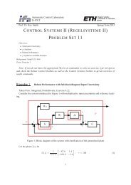
Consider the SISO system given in Fig. 1. Examine the system’s internal stability and compare with the stability of the
transfer function from r toy for the following cases, τ1,τ2,τ3 > 0:
1.
2.
3.
p(s) =
1 τ1s+1
, c(s) =
τ1s+1 τ2s+1
p(s) = τ1s+1 τ2s−1
, c(s) =
τ2s−1 (τ1s+1)(τ3s+1)
p(s) = τ1s−1 τ2s+1
, c(s) =
τ2s+1 (τ1s−1)(τ3s+1)
2 of 3

−
c(s)
du
p(s)
Figure 1: Block diagram for the discussion of Internal Stability
Exercise 4 Controllability and Observability
The linearized equations of motion for a satellite are
where
and
˙x(t) = Ax(t)+Bu(t)
y(t) = Cx(t)
⎡
0
⎢
A = ⎢3ω
⎣
1 0 0
2
0
0
0
⎤ ⎡ ⎤
0 0
0 2ω⎥
⎢
⎥
0 1 ⎦ , B = ⎢1
0 ⎥
⎣0
0⎦
, C =
0 −2ω 0 0 0 1
u =
u1
u2
, y =
dy
1 0 0 0
0 0 1 0
The inputs u1 and u2 are the radial and tangential thrusts, the state variables x1 and x3 are the radial and angular deviations
from the reference (circular) orbit and the outputs y1 and y2 are the radial and angular measurements, respectively.
Forω = 1, show that
1. The system is controllable using both control inputs.
2. The system is controllable using only a single input. Which one is it?
3. The system is observable using both measurements.
4. That the system is observable using only one measurement. Which one is it?
3 of 3
y1
y2
.
y