Model Predictive Control
Model Predictive Control
Model Predictive Control

Create successful ePaper yourself
Turn your PDF publications into a flip-book with our unique Google optimized e-Paper software.
<strong>Predictive</strong> <strong>Control</strong><br />
for linear and hybrid systems<br />
F. Borrelli, A. Bemporad, M. Morari<br />
February 23, 2011
to Maryan, Federica and Marina<br />
and all our families<br />
i
ii<br />
Preface<br />
Dynamic optimization has become a standard tool for decision making in a wide<br />
range of areas. The search for the most fuel-efficient strategy to send a rocket into<br />
orbit or the most economical way to start-up a chemical production facility can<br />
be expressed as dynamic optimization problems that are solved almost routinely<br />
nowadays.<br />
The basis for these dynamic optimization problems is a dynamic model, for<br />
example,<br />
x(k + 1) = g(x(k), u(k)), x(0) = x0<br />
that describes the evolution of the state x(k) with time, starting from the initial<br />
condition x(0), as it is affected by the manipulated input u(k). Here g(x, u) is<br />
some nonlinear function. Throughout the book we are assuming that this discretetime<br />
description, i.e., the model of the underlying system is available. The goal<br />
of the dynamic optimization procedure is to find the vector of manipulated inputs<br />
UN = [u(0) ′ , ..., u(N −1) ′ ] ′ such that the objective function is optimized over some<br />
time horizon N, typically<br />
minUN<br />
N−1 <br />
k=0<br />
q(x(k), u(k)) + p(x(N))<br />
The terms q(x, u) and and p(x) are referred to as the stage cost and terminal cost,<br />
respectively. Many practical problems can be put into this form and many algorithms<br />
and software packages are available to determine the optimal solution vector<br />
U ∗ N<br />
, the optimizer. The various algorithms exploit the structure of the particular<br />
problem, e.g., linearity and convexity, so that even large problems described by<br />
complex models and involving many degrees of freedom can be solved efficiently<br />
and reliably.<br />
One difficulty with this idea is that, in practice, the sequence of u(0), u(1), ...,<br />
which is obtained by this procedure cannot be simply applied. The model of the<br />
system predicting its evolution is usually inaccurate and the system may be affected<br />
by external disturbances that may cause its path to deviate significantly from the<br />
one that is predicted. Therefore, it is common practice to measure the state after<br />
some time period, say one time step, and to solve the dynamic optimization problem<br />
again, starting from the measured state x(1) as the new initial condition. This<br />
feedback of the measurement information to the optimization endows the whole<br />
procedure with a robustness typical of closed-loop systems.<br />
What we have described above is usually referred to as <strong>Model</strong> <strong>Predictive</strong> <strong>Control</strong><br />
(MPC), but other names like Open Loop Optimal Feedback and Reactive Scheduling<br />
have been used as well. Over the last 25 years MPC has evolved to dominate<br />
the process industry, where it has been employed for thousands of problems [210].<br />
The popularity of MPC stems from the fact that the resulting operating strategy<br />
respects all the system and problem details, including interactions and constraints,<br />
which would be very hard to accomplish in any other way.<br />
Indeed, often MPC is used for the regulatory control of large multivariable<br />
linear systems with constraints, where the objective function is not related to an<br />
economical objective, but is simply chosen in a mathematically convenient way,
namely quadratic in the states and inputs, to yield a “good” closed-loop response.<br />
Again, there is no other controller design method available today for such systems,<br />
that provides constraint satisfaction and stability guarantees.<br />
One limitation of MPC is that running the optimization algorithm on-line at<br />
each time step requires substantial time and computational resources, which are<br />
generally available in a large “slow” chemical production facility, but may not<br />
be available for the control of a system installed in an automobile that must be<br />
inexpensive and where the sampling time is in the range of milliseconds. In this<br />
case it would be desirable to have the result of the optimization pre-computed<br />
and stored for each x in the form of a look-up table or as an algebraic function<br />
u(k) = f(x(k)) which can be easily evaluated.<br />
In other words, we want to determine the (generally nonlinear) feedback control<br />
law f(x) that generates the optimal u(k) = f(x(k)) explicitly and not just implicitly<br />
as the result of an optimization problem. It requires the solution of the Bellman<br />
equation and has been a long standing problem in optimal control. A clean simple<br />
solution exists only in the case of linear systems with a quadratic objective function,<br />
where the optimal controller turns out to be a linear function of the state (Linear<br />
Quadratic Regulator, LQR). For all other cases a solution of the Bellman equation<br />
was considered prohibitive except for systems of dimension 2 or 3, where a look-up<br />
table can be generated by gridding the state space and solving the optimization<br />
problem off-line for each grid point.<br />
generally, hybrid systems. The major new contribution of this book is to show<br />
how the nonlinear optimal feedback controller can be calculated efficiently for some<br />
important classes of systems, namely linear systems with constraints and switched<br />
linear systems or, more generally, hybrid systems. Traditionally, the design of<br />
feedback controllers for linear systems with constraints, for example anti-windup<br />
techniques, was ad hoc requiring both much experience and trial and error. Though<br />
significant progress has been achieved on anti-windup schemes over the last decade,<br />
these techniques deal with input constraints only and cannot be extended easily.<br />
The classes of constrained linear systems and linear hybrid systems treated in<br />
this book cover many, if not most, practical problems. The new design techniques<br />
hold the promise to lead to better performance and a dramatic reduction in the<br />
required engineering effort.<br />
The book is structured into four parts. Chapters marked with a star (∗) are<br />
consider “advanced” material and can be skipped without compromising the understanding<br />
of the fundamental concepts presented in the book.<br />
• In the first part of the book (Part I) we recall the main concepts and results of<br />
convex and discrete optimization.Our intent is to provide only the necessary<br />
background for the understanding of the rest of the book. The material of this<br />
part has been extracted from the following books and lecture notes: “Convex<br />
optimization” by Boyd and Vandenberghe [56], “Nonlinear Programming<br />
Theory and Algorithms” by Bazaraa, Sherali, Shetty [23], “LMIs in <strong>Control</strong>”<br />
by Scherer and Weiland [223] and “Lectures on Polytopes” by Ziegler [100].<br />
Continuous problems as well Integer and Mixed-Integer problems are presented<br />
in Chapter 1. Chapter 2 discusses the classical results of Lagrange<br />
duality. Since polyhedra are the fundamental geometric objects used in this<br />
iii
iv<br />
book, in Chapter 3 we introduce the main definitions and the algorithms<br />
which describe standard operations on polyhedra. Part I closes with Chapter<br />
4 where Linear and Quadratic programs are presented together with their<br />
properties and some fundamental results.<br />
• The second part of the book (Part II) is a self-contained introduction to<br />
multi-parametric programming. In our framework, parametric programming<br />
is the main technique used to study and compute state feedback optimal<br />
control laws. In fact, we formulate the finite time optimal control problems<br />
as mathematical programs where the input sequence is the optimization vector.<br />
Depending on the dynamical model of the system, the nature of the<br />
constraints, and the cost function used, a different mathematical program is<br />
obtained. The current state of the dynamical system enters the cost function<br />
and the constraints as a parameter that affects the solution of the mathematical<br />
program. We study the structure of the solution as this parameter changes<br />
and we describe algorithms for solving multi-parametric linear, quadratic and<br />
mixed integer programs. They constitute the basic tools for computing the<br />
state feedback optimal control laws for these more complex systems in the<br />
same way as algorithms for solving the Riccati equation are the main tools for<br />
computing optimal controllers for linear systems. In Chapter 5 we introduce<br />
the concept of multiparametric programming and we recall the main results<br />
of nonlinear multiparametric programming. Then, in Chapter 6 we describe<br />
three algorithms for solving multiparametric linear programs (mp-LP), multiparametric<br />
quadratic programs (mp-QP) and multiparametric mixed-integer<br />
linear programs (mp-MILP).<br />
• In the third part of the book (Part III) we introduce the general class of<br />
optimal control problem studied in the book. Chapter 7 contains the basic<br />
definitions and essential concepts. Chapter 8 presents standard results on<br />
Linear Quadratic Optimal <strong>Control</strong> while Chapter 9 studies unconstrained<br />
optimal control problems for linear systems with cost functions based on 1<br />
and ∞ norms.<br />
• In the fourth part of the book (Part IV) we focus on linear systems with<br />
polyhedral constraints on inputs and states. We study finite time and infinite<br />
time optimal control problems with cost functions based on 2, 1 and ∞<br />
norms. in Chapter 10 we demonstrate that the solution to all these optimal<br />
control problems can be expressed as a piecewise affine state feedback law.<br />
Moreover, the optimal control law is continuous and the value function is<br />
convex and continuous. The results form a natural extension of the theory<br />
of the Linear Quadratic Regulator to constrained linear systems. Chapter 10<br />
also presents a self-contained introduction to invariant set theory as well as<br />
dynamic programming for constrained systems.<br />
Chapter 11 presents the concept of <strong>Model</strong> <strong>Predictive</strong> <strong>Control</strong>. Classical feasibility<br />
and stability issues are shown through simple examples and explained<br />
by using invariant set methods. Finally we show how they can be solved with<br />
a proper choice of terminal constraints and cost function.
Chapter 12 addresses the robustness of the optimal control laws. We discuss<br />
min-max control problems for uncertain linear systems with polyhedral constraints<br />
on inputs and states and present an approach to compute their state<br />
feedback solutions. Robustness is achieved against additive norm-bounded<br />
input disturbances and/or polyhedral parametric uncertainties in the statespace<br />
matrices.<br />
The result in Chapter 10 have important consequences for the implementation<br />
of MPC laws. Precomputing off-line the explicit piecewise affine feedback<br />
policy reduces the on-line computation for the receding horizon control law to<br />
a function evaluation, therefore avoiding the on-line solution of a mathematical<br />
program. In Chapter 13 the evaluation of the piecewise affine optimal<br />
feedback policy is carefully studied and we present algorithms to reduce its<br />
storage demands and computational complexity.<br />
• In the fifth part of the book (Part V) we focus on linear hybrid systems. We<br />
give an introduction to the different formalisms used to model hybrid systems<br />
focusing on computation-oriented models (Chapter 14). In Chapter 15 we<br />
study finite time optimal control problems with cost functions based on 2, 1<br />
and ∞ norms. The optimal control law is shown to be, in general, piecewise<br />
affine over non-convex and disconnected sets. Along with the analysis of the<br />
solution properties we present algorithms that efficiently compute the optimal<br />
control law for all the considered cases.<br />
Berkeley Francesco Borrelli<br />
Trento Alberto Bemporad<br />
Zurich Manfred Morari<br />
May 2010<br />
v
vi<br />
Acknowledgements<br />
Large part of the material presented in this book is extracted from the work of<br />
the authors Francesco Borrelli, Alberto Bemporad and Manfred Morari. Several<br />
sections have also been extracted from the PhD Theses of Miroslav Baric, Mato<br />
Baotic, Fabio Torrisi, Domenico Mignone, Pascal Grieder, Eric Kerrigan, Tobias<br />
Geyer and Frank J. Christophersen. A special tanks goes to Michal Kvasnica,<br />
Stefan Richter and Thomas Besselmann for their invaluable help on the examples<br />
construction.<br />
Our gratitude also goes to the several people who have careful read preliminary<br />
versions of the book and gave us suggestions on how to improve them. They<br />
include David Mayne, Per Olof Gutman and all the students of our class on <strong>Model</strong><br />
<strong>Predictive</strong> <strong>Control</strong> (ME290J at UC Berkeley, 227-0221-00 at ETH).<br />
The authors of the book style and macros are Stephen Boyd and Lieven Vandenberghe.<br />
We are extremely grateful to Stephen and Lieven for sharing them with<br />
us.
Contents<br />
I Basics on Optimization 1<br />
1 Main Concepts 3<br />
1.1 Optimization Problems . . . . . . . . . . . . . . . . . . . . . . . . . . 3<br />
1.2 Convexity . . . . . . . . . . . . . . . . . . . . . . . . . . . . . . . . . 6<br />
2 Optimality Conditions 9<br />
2.1 Introduction . . . . . . . . . . . . . . . . . . . . . . . . . . . . . . . . 9<br />
2.2 Lagrange Duality Theory . . . . . . . . . . . . . . . . . . . . . . . . 10<br />
2.3 Complementary Slackness . . . . . . . . . . . . . . . . . . . . . . . . 13<br />
2.4 Karush-Kuhn-Tucker Conditions . . . . . . . . . . . . . . . . . . . . 14<br />
3 Polyhedra, Polytopes and Simplices 19<br />
3.1 General Set Definitions and Operations . . . . . . . . . . . . . . . . 19<br />
3.2 Polyhedra Definitions and Representations . . . . . . . . . . . . . . . 21<br />
3.3 Polytopal Complexes . . . . . . . . . . . . . . . . . . . . . . . . . . . 24<br />
3.4 Basic Operations on Polytopes . . . . . . . . . . . . . . . . . . . . . 26<br />
3.5 Operations on P-collections . . . . . . . . . . . . . . . . . . . . . . . 37<br />
4 Linear and Quadratic Optimization 45<br />
4.1 Linear Programming . . . . . . . . . . . . . . . . . . . . . . . . . . . 45<br />
4.2 Quadratic Programming . . . . . . . . . . . . . . . . . . . . . . . . . 52<br />
4.3 Mixed-Integer Optimization . . . . . . . . . . . . . . . . . . . . . . . 55<br />
II Multiparametric Programming 59<br />
5 General Results for Multiparametric Nonlinear Programs. 61<br />
5.1 General Results for Multiparametric Nonlinear Programs . . . . . . 64<br />
6 Multiparametric Programming: a Geometric Approach 73<br />
6.1 Multiparametric Programs with Linear Constraints . . . . . . . . . . 74<br />
6.2 Multiparametric Linear Programming . . . . . . . . . . . . . . . . . 77<br />
6.3 Multiparametric Quadratic Programming . . . . . . . . . . . . . . . 93<br />
6.4 Multiparametric Mixed-Integer Linear Programming . . . . . . . . . 107<br />
6.5 Multiparametric Mixed-Integer Quadratic Programming . . . . . . . 111<br />
6.6 Literature Review . . . . . . . . . . . . . . . . . . . . . . . . . . . . 112
viii Contents<br />
III Optimal <strong>Control</strong> 115<br />
7 General Formulation and Discussion 117<br />
7.1 Problem Formulation . . . . . . . . . . . . . . . . . . . . . . . . . . . 117<br />
7.2 Solution via Batch Approach . . . . . . . . . . . . . . . . . . . . . . 119<br />
7.3 Solution via Recursive Approach . . . . . . . . . . . . . . . . . . . . 120<br />
7.4 Optimal <strong>Control</strong> Problem with Infinite Horizon . . . . . . . . . . . . 122<br />
7.5 Lyapunov Stability . . . . . . . . . . . . . . . . . . . . . . . . . . . . 126<br />
8 Linear Quadratic Optimal <strong>Control</strong> 133<br />
8.1 Solution via Batch Approach . . . . . . . . . . . . . . . . . . . . . . 134<br />
8.2 Solution via Recursive Approach . . . . . . . . . . . . . . . . . . . . 135<br />
8.3 Comparison Of The Two Approaches . . . . . . . . . . . . . . . . . . 136<br />
8.4 Infinite Horizon Problem . . . . . . . . . . . . . . . . . . . . . . . . . 137<br />
8.5 Stability of the Infinite Horizon LQR . . . . . . . . . . . . . . . . . . 139<br />
9 1/∞ Norm Optimal <strong>Control</strong> 141<br />
9.1 Solution via Batch Approach . . . . . . . . . . . . . . . . . . . . . . 142<br />
9.2 Solution via Recursive Approach . . . . . . . . . . . . . . . . . . . . 144<br />
9.3 Comparison Of The Two Approaches . . . . . . . . . . . . . . . . . . 146<br />
9.4 Infinite Horizon Problem . . . . . . . . . . . . . . . . . . . . . . . . . 147<br />
IV Constrained Optimal <strong>Control</strong> of Linear Systems 151<br />
10 Constrained Optimal <strong>Control</strong> 153<br />
10.1 Invariant Sets . . . . . . . . . . . . . . . . . . . . . . . . . . . . . . . 154<br />
10.2 Constrained Optimal <strong>Control</strong> Problem Formulation . . . . . . . . . . 164<br />
10.3 Feasible Solutions . . . . . . . . . . . . . . . . . . . . . . . . . . . . . 166<br />
10.4 State Feedback Solution, 2-Norm Case . . . . . . . . . . . . . . . . . 171<br />
10.5 State Feedback Solution, 1-Norm and ∞-Norm Case . . . . . . . . . 179<br />
10.6 State-Feedback Solution, Minimum-Time <strong>Control</strong> . . . . . . . . . . . 188<br />
11 Receding Horizon <strong>Control</strong> 195<br />
11.1 Introduction . . . . . . . . . . . . . . . . . . . . . . . . . . . . . . . . 196<br />
11.2 RHC Implementation . . . . . . . . . . . . . . . . . . . . . . . . . . 197<br />
11.3 RHC Main Issues . . . . . . . . . . . . . . . . . . . . . . . . . . . . . 203<br />
11.4 State Feedback Solution of RHC, 2-Norm Case . . . . . . . . . . . . 209<br />
11.5 State Feedback Solution of RHC, 1, ∞-Norm Case . . . . . . . . . . 214<br />
11.6 RHC Extensions . . . . . . . . . . . . . . . . . . . . . . . . . . . . . 218<br />
11.7 Offset-Free Reference Tracking . . . . . . . . . . . . . . . . . . . . . 218<br />
11.8 Literature Review . . . . . . . . . . . . . . . . . . . . . . . . . . . . 226<br />
12 Constrained Robust Optimal <strong>Control</strong> 233<br />
12.1 Introduction . . . . . . . . . . . . . . . . . . . . . . . . . . . . . . . . 234<br />
12.2 Robust Invariant Sets . . . . . . . . . . . . . . . . . . . . . . . . . . 234<br />
12.3 Problem Formulation . . . . . . . . . . . . . . . . . . . . . . . . . . . 246<br />
12.4 Feasible Solutions . . . . . . . . . . . . . . . . . . . . . . . . . . . . . 250
Contents ix<br />
12.5 State Feedback Solution, 1-Norm and ∞-Norm Case . . . . . . . . . 255<br />
12.6 Parametrizations of the <strong>Control</strong> Policies . . . . . . . . . . . . . . . . 260<br />
12.7 Example . . . . . . . . . . . . . . . . . . . . . . . . . . . . . . . . . . 263<br />
12.8 Robust Receding Horizon <strong>Control</strong> . . . . . . . . . . . . . . . . . . . . 264<br />
12.9 Literature Review . . . . . . . . . . . . . . . . . . . . . . . . . . . . 266<br />
13 On-line <strong>Control</strong> Computation 267<br />
13.1 Introduction . . . . . . . . . . . . . . . . . . . . . . . . . . . . . . . . 268<br />
13.2 Efficient On-Line Algorithms . . . . . . . . . . . . . . . . . . . . . . 269<br />
13.3 Example . . . . . . . . . . . . . . . . . . . . . . . . . . . . . . . . . . 278<br />
13.4 Literature Review . . . . . . . . . . . . . . . . . . . . . . . . . . . . 279<br />
V Constrained Optimal <strong>Control</strong> of Hybrid Systems 281<br />
14 <strong>Model</strong>s of Hybrid Systems 283<br />
14.1 Hybrid models . . . . . . . . . . . . . . . . . . . . . . . . . . . . . . 283<br />
14.2 Piecewise Affine Systems . . . . . . . . . . . . . . . . . . . . . . . . . 284<br />
14.3 Discrete Hybrid Automata . . . . . . . . . . . . . . . . . . . . . . . . 291<br />
14.4 Logic and Mixed-Integer Inequalities . . . . . . . . . . . . . . . . . . 296<br />
14.5 Mixed Logical Dynamical Systems . . . . . . . . . . . . . . . . . . . 299<br />
14.6 <strong>Model</strong> Equivalence . . . . . . . . . . . . . . . . . . . . . . . . . . . . 300<br />
14.7 The HYSDEL <strong>Model</strong>ing Language . . . . . . . . . . . . . . . . . . . 301<br />
14.8 Literature Review . . . . . . . . . . . . . . . . . . . . . . . . . . . . 306<br />
15 Optimal <strong>Control</strong> of Hybrid Systems 311<br />
15.1 Problem Formulation . . . . . . . . . . . . . . . . . . . . . . . . . . . 312<br />
15.2 Properties of the State Feedback Solution, 2-Norm Case . . . . . . . 314<br />
15.3 Properties of the State Feedback Solution, 1, ∞-Norm Case . . . . . 321<br />
15.4 Computation of the Optimal <strong>Control</strong> Input via Mixed Integer Programming322<br />
15.5 State Feedback Solution via Batch Approach . . . . . . . . . . . . . 324<br />
15.6 State Feedback Solution via Recursive Approach . . . . . . . . . . . 325<br />
15.7 Discontinuous PWA systems . . . . . . . . . . . . . . . . . . . . . . . 334<br />
15.8 Receding Horizon <strong>Control</strong> . . . . . . . . . . . . . . . . . . . . . . . . 335<br />
Bibliography 341
x Contents<br />
Symbols and Acronyms<br />
Logic Operators and Functions<br />
A ⇒ B A implies B, i.e., if A is true then B must be true<br />
A ⇔ B A implies B and B implies A, i.e., A is true if and only if (iff) B is true<br />
Sets<br />
R (R+) Set of (non-negative) real numbers<br />
N (N+) Set of (non-negative) integers<br />
R n Set of real vectors with n elements<br />
R n×m Set of real matrices with n rows and m columns<br />
Algebraic Operators and Matrices<br />
[a, b] depending on the context: a closed interval in R or a row vector<br />
A ′ Transpose of matrix A<br />
A−1 Inverse of matrix A<br />
det(A) Determinant of matrix A<br />
A ≻ ()0 A symmetric positive (semi)definite matrix, x ′ Ax > (≥)0, ∀x = 0<br />
A ≺ ()0 A symmetric negative (semi)definite matrix, x ′ Ax < (≤)0, ∀x = 0.<br />
i-th row of matrix A<br />
Ai<br />
xi<br />
i-th element of vector x<br />
x ∈ Rn , x > 0 (x ≥ 0)<br />
x ∈ R<br />
true iff xi > 0 (xi ≥ 0) ∀ i = 1, . . .,n<br />
n , x < 0 (x ≤ 0) true iff xi < 0 (xi ≤ 0) ∀ i = 1, . . .,n<br />
|x|, x ∈ R absolute value of x<br />
x<br />
x2<br />
Any vector norm of x<br />
Euclidian norm of vector x ∈ Rn , x2 = <br />
x1<br />
n<br />
i=1 |xi| 2<br />
Sum of absolute elements of vector x ∈ Rn , x1 := n i=1 |xi|<br />
x∞<br />
Largest absolute value of the vector x ∈ Rn , x∞ := maxi∈{1,...,n} |xi|<br />
S∞<br />
The matrix ∞-norm of S ∈ Cm×nz ,i.e., S∞ = max1≤i≤m<br />
S1<br />
The matrix 1-norm of S ∈ Cm×nz , i.e., S1 = max1≤j≤nz<br />
I Identity matrix<br />
1 Vector of ones, 1 = [1 1 . . . 1] ′<br />
0 Vector of zeros, 0 = [0 0 . . . 0] ′<br />
nz j=1 |si,j|<br />
m i=1 |si,j|
Contents xi<br />
Set Operators and Functions<br />
∅ The empty set<br />
|P| The cardinality of P, i.e., the number of elements in P<br />
P ∩ Q Set intersection P ∩ Q = {x : x ∈ P and x ∈ Q}<br />
<br />
P ∪ Q<br />
r∈{1,...,R}<br />
Set union P ∪ Q = {x : x ∈ P or x ∈ Q}<br />
Pr Union of R sets Pr, i.e. <br />
r∈{1,...,R} Pr<br />
P<br />
= {x : x ∈ P0 or . . . or x ∈ PR}<br />
c Complement of the set P, Pc = {x : x /∈ P}<br />
P \ Q Set difference P \ Q = {x : x ∈ P and x /∈ Q}<br />
P ⊆ Q The set P is a subset of Q, x ∈ P ⇒ x ∈ Q<br />
P ⊂ Q The set P is a strict subset of Q, x ∈ P ⇒ x ∈ Q and ∃x ∈ (Q \ P)<br />
P ⊇ Q The set P is a superset of Q<br />
P ⊃ Q The set P is a strict superset of Q<br />
P ⊖ Q Pontryagin difference P ⊖ Q = {x : x + q ∈ P, ∀q ∈ Q}<br />
P ⊕ Q Minkowski sum P ⊕ Q = {x + q : x ∈ P, q ∈ Q}<br />
∂P The boundary of P<br />
int(P) The interior of P, i.e. int(P) = P \ ∂P<br />
f(x) with abuse of notation denotes the value of the function f in x or the function f, f : x → f(x). T<br />
: “such that”<br />
Acronyms<br />
ARE Algebraic Riccati Equation<br />
BMI Bilinear Matrix Inequality<br />
CLQR Constrained Linear Quadratic Regulator<br />
CFTOC Constrained Finite Time Optimal <strong>Control</strong><br />
CITOC Constrained Infinite Time Optimal <strong>Control</strong><br />
DP Dynamic Program(ming)<br />
LMI Linear Matrix Inequality<br />
LP Linear Program(ming)<br />
LQR Linear Quadratic Regulator<br />
LTI Linear Time Invariant<br />
MILP Mixed Integer Linear Program<br />
MIQP Mixed Integer Quadratic Program<br />
MPC <strong>Model</strong> <strong>Predictive</strong> <strong>Control</strong><br />
mp-LP multi-parametric Linear Program<br />
mp-QP multi-parametric Quadratic Program<br />
PWA Piecewise Affine (See Definition 3.7)<br />
PPWA Piecewise Affine on Polyhedra (See Definition 3.8)<br />
PWP Piecewise Polynomial<br />
PWQ Piecewise Quadratic<br />
QP Quadratic Program(ming)<br />
RHC Receding Horizon <strong>Control</strong><br />
rhs right-hand side<br />
SDP Semi Definite Program(ming)
xii Contents<br />
Dynamical Systems<br />
x(k) Measurement/Estimation of state x at time k<br />
Predicted value of state x at time k, given a measurement x(0)<br />
xk<br />
x + Successor of vector x, i.e. if x = x(k) then x + = x(k + 1)<br />
F∞<br />
O∞<br />
C∞<br />
K∞<br />
OLQR ∞<br />
Minimal robust positively invariant set<br />
Maximal robust positively invariant set<br />
Maximal robust control invariant set<br />
Maximal robust stabilizable set<br />
Maximal positively invariant set O∞ for LTI system under LQR feedback
Part I<br />
Basics on Optimization
Chapter 1<br />
Main Concepts<br />
In this Chapter we introduce the main concepts and definitions of mathematical<br />
programming theory.<br />
1.1 Optimization Problems<br />
An optimization problem is generally formulated as<br />
infz f(z)<br />
subj. to z ∈ S ⊆ Z<br />
(1.1)<br />
where the vector z collects the decision variables, Z is the domain of the decision<br />
variables, S ⊆ Z is the set of feasible or admissible decisions. The function f :<br />
Z → R assigns to each decision z a cost f(z) ∈ R. We will often use the following<br />
shorter form of problem (1.1)<br />
inf f(z) (1.2)<br />
z∈S⊆Z<br />
Solving problem (1.2) means to compute the least possible cost J ∗<br />
J ∗ inf<br />
z∈S f(z)<br />
The number J ∗ is the optimal value of problem (1.2), i.e., the greatest lower bound<br />
of f(z) over the set S:<br />
f(z) ≥ J ∗ , ∀z ∈ S and (∃¯z ∈ S : f(¯z) = J ∗ or ∀ε > 0 ∃z ∈ S : f(z) ≤ J ∗ + ε)<br />
If J ∗ = −∞ we say that the problem is unbounded below. If the set S is empty<br />
then the problem is said to be infeasible and we set J ∗ = +∞ by convention. If<br />
S = Z the problem is said to be unconstrained.<br />
In general, one is also interested in finding an optimal solution, that is in finding<br />
a decision whose associated cost equals the optimal value, i.e., z ∗ ∈ S with f(z ∗ ) =<br />
J ∗ . If such z ∗ exists, then we rewrite problem (1.2) as<br />
J ∗ = min f(z) (1.3)<br />
z∈S
4 1 Main Concepts<br />
and z ∗ is called optimizer or global optimizer. The set of all optimal solutions is<br />
denoted by<br />
argmin z∈S f(z) {z ∈ S : f(z) = J ∗ }.<br />
The problem of determining whether the set of feasible decisions is empty and, if<br />
not, to find a point which is feasible, is called feasibility problem.<br />
1.1.1 Continuous Problems<br />
In continuous optimization the problem domain Z is a subset of the finite-dimensional<br />
Euclidian vector-space R s and the subset of admissible vectors is defined through<br />
a list of real-valued functions:<br />
infz f(z)<br />
subj. to gi(z) ≤ 0 for i = 1, . . .,m<br />
hi(z) = 0<br />
z ∈ Z<br />
for i = 1, . . . , p<br />
(1.4)<br />
where f, g1, . . .,gm, h1, . . .,hp are real-valued functions defined over R s , i.e., f :<br />
R s → R, gi : R s → R, hi : R s → R. The domain Z is the intersection of the<br />
domains of the cost and constraint functions:<br />
Z = {z ∈ R s : z ∈ dom f, z ∈ dom gi, i = 1, . . .,m, z ∈ dom hi, i = 1, . . .,p}<br />
(1.5)<br />
In the sequel we will consider the constraint z ∈ Z implicit in the optimization<br />
problem and often omit it. Problem (1.4) is unconstrained if m = p = 0.<br />
The inequalities gi(z) ≤ 0 are called inequality constraints and the equations<br />
hi(z) = 0 are called equality constraints. A point ¯z ∈ R s is feasible for problem (1.4)<br />
if: (i) it belongs to Z, (ii) it satisfies all inequality and equality constraints, i.e.,<br />
gi(¯z) ≤ 0, i = 1, . . .,m, hi(¯z) = 0, i = 1, . . .,p. The set of feasible vectors is<br />
S = {z ∈ R s : z ∈ Z, gi(z) ≤ 0, i = 1, . . .,m, hi(z) = 0, i = 1, . . .,p}. (1.6)<br />
Problem (1.4) is a continuous finite-dimensional optimization problem (since<br />
Z is a finite-dimensional Euclidian vector space). We will also refer to (1.4) as<br />
a nonlinear mathematical program or simply nonlinear program. Let J ∗ be the<br />
optimal value of problem (1.4). An optimizer, if it exists, is a feasible vector z∗ with f(z ∗ ) = J ∗ .<br />
A feasible point ¯z is locally optimal for problem (1.4) if there exists an R ≻ 0<br />
such that<br />
f(¯z) = infz f(z)<br />
subj. to gi(z) ≤ 0 for i = 1, . . .,m<br />
hi(z) = 0 for i = 1, . . .,p (1.7)<br />
z − ¯z ≤ R<br />
z ∈ Z<br />
Roughly speaking, this means that ¯z is the minimizer of f(z) in a feasible neighborhood<br />
of ¯z defined by z − ¯z ≤ R. The point ¯z is called local optimizer.
1.1 Optimization Problems 5<br />
Active, Inactive and Redundant Constraints<br />
Consider a feasible point ¯z. We say that the i-th inequality constraint gi(z) ≤ 0 is<br />
active at ¯z if gi(¯z) = 0. If gi(¯z) < 0 we say that the constraint gi(z) ≤ 0 is inactive<br />
at ¯z. Equality constraints are always active for all feasible points.<br />
We say that a constraint is redundant if removing it from the list of constraints<br />
does not change the feasible set S. This implies that removing a redundant constraint<br />
from problem (1.4) does not change its solution.<br />
Problems in Standard Forms<br />
Optimization problems can be cast in several forms. In this book we use the<br />
form (1.4) where we adopt the convention to minimize the cost function and to<br />
have the right-hand side of the inequality and equality constraints equal to zero.<br />
Any problem in a different form (e.g., a maximization problem or a problem with<br />
“box constraints”) can be transformed and arranged into this form. The interested<br />
reader is referred to Chapter 4 of [56] for a detailed discussion on transformations<br />
of optimization problems into different standard forms.<br />
Eliminating Equality Constraints<br />
Often in this book we will restrict our attention to problems without equality<br />
constraints, i.e., p = 0<br />
infz f(z)<br />
subj. to gi(z) ≤ 0 for i = 1, . . .,m<br />
(1.8)<br />
The simplest way to remove equality constraints is to replace them with two inequalities<br />
for each equality, i.e., hi(z) = 0 is replaced by hi(z) ≤ 0 and −hi(z) ≤ 0.<br />
Such a method, however, can lead to poor numerical conditioning and may ruin<br />
the efficiency and accuracy of a numerical solver.<br />
If one can explicitly parameterize the solution of the equality constraint hi(z) =<br />
0, then the equality constraint can be eliminated from the problem. This process<br />
can be described in a simple way for linear equality constraints. Assume the equality<br />
constraints to be linear, Az − b = 0, with A ∈ R p×s . If Az = b is inconsistent<br />
then the problem is infeasible. The general solution of the equation Az = b can be<br />
expressed as z = Fx + x0 where F is a matrix of full rank whose spanned space<br />
coincides with the null space of the A matrix, i.e., R(F) = N(A), F ∈ R s×k ,<br />
where k is the dimension of the null space of A. The variable x ∈ R k is the new<br />
optimization variable and the original problem becomes<br />
infx f(Fx + x0)<br />
subj. to gi(Fx + x0) ≤ 0 for i = 1, . . .,m<br />
(1.9)<br />
We want to point out that in some cases the elimination of equality constraints<br />
can make the problem harder to analyze and understand and can make a solver<br />
less efficient. In large problems it can destroy useful structural properties of the<br />
problem such as sparsity. Some advanced numerical solvers perform elimination<br />
automatically.
6 1 Main Concepts<br />
Problem Description<br />
The functions f, gi and hi can be available in analytical form or can be described<br />
through an oracle model (also called “black box” or “subroutine” model). In an<br />
oracle model f, gi and hi are not known explicitly but can be evaluated by querying<br />
the oracle. Often the oracle consists of subroutines which, called with the argument<br />
z, return f(z), gi(z) and hi(z) and their gradients ∇f(z), ∇gi(z), ∇hi(z). In<br />
the rest of the book we assume that analytical expressions of the cost and the<br />
constraints of the optimization problem are available.<br />
1.1.2 Integer and Mixed-Integer Problems<br />
If the decision set Z in the optimization problem (1.2) is finite, then the optimization<br />
problem is called combinatorial or discrete. If Z ⊆ {0, 1} s , then the problem<br />
is said to be integer.<br />
If Z is a subset of the Cartesian product of an integer set and a real Euclidian<br />
space, i.e., Z ⊆ {[zc, zb] : zc ∈ R sc , zb ∈ {0, 1} sb }, then the problem is said to be<br />
mixed-integer. The standard formulation of a mixed-integer nonlinear program is<br />
inf [zc,zb] f(zc, zb)<br />
subj. to gi(zc, zb) ≤ 0 for i = 1, . . .,m<br />
hi(zc, zb) = 0 for i = 1, . . .,p<br />
zc ∈ R sc , zb ∈ {0, 1} sb<br />
[zc, zb] ∈ Z<br />
(1.10)<br />
where f, g1, . . .,gm, h1, . . .,hp are real-valued functions defined over Z.<br />
For combinatorial, integer and mixed-integer optimization problems all definitions<br />
introduced in the previous section apply.<br />
1.2 Convexity<br />
A set S ∈ R s is convex if<br />
λz1 + (1 − λ)z2 ∈ S for all z1, z2 ∈ S, λ ∈ [0, 1].<br />
A function f : S → R is convex if S is convex and<br />
f(λz1 + (1 − λ)z2) ≤ λf(z1) + (1 − λ)f(z2)<br />
for all z1, z2 ∈ S, λ ∈ [0, 1].<br />
A function f : S → R is strictly convex if S is convex and<br />
f(λz1 + (1 − λ)z2) < λf(z1) + (1 − λ)f(z2)<br />
for all z1, z2 ∈ S, λ ∈ (0, 1).<br />
A function f : S → R is concave if S is convex and −f is convex.
1.2 Convexity 7<br />
Operations preserving convexity<br />
Various operations preserve convexity of functions and sets. A detailed list can<br />
be found in Chapter 3.2 of [56]. A few operations used in this book are reported<br />
below.<br />
1. The intersection of an arbitrary number of convex sets is a convex set:<br />
if S1, S2, . . . , Sk are convex, then S1 ∩ S2 ∩ . . . ∩ Sk is convex.<br />
This property extends to the intersection of an infinite number of sets:<br />
if Sn is convex foralln ∈ N+ then <br />
Sn is convex.<br />
n∈N+<br />
The empty set is convex because it satisfies the definition of convexity.<br />
2. The sub-level sets of a convex function f on S are convex:<br />
if f(z) is convex then Sα {z ∈ S : f(z) ≤ α} is convex ∀α.<br />
3. If f1, . . . , fN are convex functions, then N<br />
i=1 αifi is a convex function for all<br />
αi ≥ 0, i = 1, . . .,N.<br />
4. The composition of a convex function f(z) with an affine map z = Ax + b<br />
generates a convex function f(Ax + b) of x:<br />
if f(z) is convex then f(Ax + b) is convex on{x : Ax + b ∈ dom(f)}<br />
5. Suppose f(x) = h(g(x)) = h(g1(x), . . . , gk(x)) with h : R k → R, gi : R s → R.<br />
Then,<br />
(a) f is convex if h is convex, h is nondecreasing in each argument, and gi<br />
are convex,<br />
(b) f is convex if h is convex, h is nonincreasing in each argument, and gi<br />
are concave,<br />
(c) f is concave if h is concave, h is nondecreasing in each argument, and<br />
gi are concave.<br />
6. The pointwise maximum of a set of convex functions is a convex function:<br />
f1(z), . . .,fk(z) convex functions ⇒ f(z) = max{f1(z), . . .,fk(z)} is a convex function.<br />
Linear and quadratic convex functions<br />
The following convex functions will be used extensively in this book:<br />
1. A linear function f(z) = c ′ z + d is both convex and concave.<br />
2. A quadratic function f(z) = z ′ Qz + 2r ′ z + s is convex if and only if Q 0.<br />
3. A quadratic function f(z) = z ′ Qz + 2r ′ z + s is strictly convex if and only if<br />
Q ≻ 0.
8 1 Main Concepts<br />
Convex optimization problems<br />
The standard optimization problem (1.4) is said to be convex if the cost function f<br />
is convex on Z and S is a convex set. A fundamental property of convex optimization<br />
problems is that local optimizers are also global optimizers. This is proven in<br />
the next proposition.<br />
Proposition 1.1 Consider a convex optimization problem and let ¯z be a local optimizer.<br />
Then, ¯z is a global optimizer.<br />
Proof: By hypothesis ¯z is feasible and there exists R such that<br />
f(¯z) = inf{f(z) : gi(z) ≤ 0 i = 1, . . .,m, hi(z) = 0, i = 1, . . .,p z − ¯z ≤ R}.<br />
(1.11)<br />
Now suppose that ¯z is not globally optimal. Then, there exist a feasible y such<br />
that f(y) < f(¯z), which implies that y − ¯z > R. Now consider the point z given<br />
by<br />
z = (1 − θ)¯z + θy, θ =<br />
R<br />
2y − ¯z .<br />
Then z − ¯z = R/2 < R and by convexity of the feasible set z is feasible. By<br />
convexity of the cost function f<br />
f(z) ≤ (1 − θ)f(¯z) + θf(y) < f(¯z),<br />
which contradicts (1.11). ✷<br />
Proposition 1.1 does not make any statement about the existence of a solution<br />
to problem (1.4). It merely states that all local minima of problem (1.4) are also<br />
global minima. For this reason, convexity plays a central role in the solution<br />
of continuous optimization problems. It suffices to compute a local minimum to<br />
problem (1.4) to determine its global minimum. Convexity also plays a major role<br />
in most non-convex optimization problems which are solved by iterating between<br />
the solutions of convex sub-problems.<br />
It is difficult to determine whether the feasible set S of the optimization problem<br />
(1.4) is convex or not except in special cases. For example, if the functions<br />
g1(z), . . .,gm(z) are convex and all the hi(z) (if any) are affine in z, then the feasible<br />
region S in (1.6) is an intersection of convex sets and therefore convex. Moreover<br />
there are non-convex problems which can be transformed into convex problems<br />
through a change of variables and manipulations on cost and constraints. The discussion<br />
of this topic goes beyond the scope of this overview on optimization. The<br />
interested reader is referred to [56].<br />
Remark 1.1 With the exception of trivial cases, integer and mixed-integer optimization<br />
problems are always non-convex problems because {0, 1} is not a convex set.
Chapter 2<br />
Optimality Conditions<br />
2.1 Introduction<br />
In general, an analytical solution to problem (1.4), restated below, does not exist.<br />
infz f(z)<br />
subj. to gi(z) ≤ 0 for i = 1, . . .,m<br />
hi(z) = 0<br />
z ∈ Z<br />
for i = 1, . . .,p<br />
(2.1)<br />
Solutions are usually computed by recursive algorithms which start from an initial<br />
guess z0 and at step k generate a point zk such that the sequence {f(zk)}k=0,1,2,...<br />
converges to J ∗ as k increases. These algorithms recursively use and/or solve<br />
conditions for optimality, i.e., analytical conditions that a point z must satisfy in<br />
order to be an optimizer. For instance, for convex, unconstrained optimization<br />
problems with a smooth cost function the best known optimality criterion requires<br />
the gradient to vanish at the optimizer, i.e., z is an optimizer if and only if ∇f(z) =<br />
0.<br />
Next we will briefly summarize necessary and sufficient optimality conditions<br />
for unconstrained optimization problems.<br />
Necessary conditions (unconstrained problem)<br />
Theorem 2.1 Suppose that f : R s → R is differentiable at ¯z. If there exists a<br />
vector d such that ∇f(¯z) ′ d < 0, then there exists a δ > 0 such that f(¯z+λd) <<br />
f(¯z) for all λ ∈ (0, δ).<br />
The vector d in the theorem above is called descent direction. In a given point<br />
¯z a descent direction d satisfies the condition ∇f(¯z) ′ d < 0. Theorem 2.1<br />
states that if a descent direction exists at a point ¯z, then it is possible to<br />
move from ¯z towards a new point ˜z whose associated cost f(˜z) is lower than<br />
f(¯z). The smaller ∇f(¯z) ′ d is the smaller will be the cost at the new point<br />
f(˜z). The direction of steepest descent ds at a given point ¯z is defined as the<br />
normalized direction where ∇f(¯z) ′ ds < 0 is minimized. The direction ds of<br />
steepest descent is ds = − ∇f(¯z)<br />
∇f(¯z) .
10 2 Optimality Conditions<br />
Two corollaries of Theorem 2.1 are stated next.<br />
Corollary 2.1 Suppose that f : R s → R is differentiable at ¯z. If ¯z is a local<br />
minimizer, then ∇f(¯z) = 0.<br />
Corollary 2.2 Suppose that f : R s → R is twice differentiable at ¯z. If ¯z<br />
is a local minimizer, then ∇f(¯z) = 0 and the Hessian ∇ 2 f(¯z) is positive<br />
semidefinite.<br />
Sufficient condition (unconstrained problem)<br />
Theorem 2.2 Suppose that f : R s → R is twice differentiable at ¯z. If<br />
∇f(¯z) = 0 and the Hessian of f(z) at ¯z is positive definite, then ¯z is a<br />
local minimizer<br />
Necessary and sufficient condition (unconstrained problem)<br />
Theorem 2.3 Suppose that f : R s → R is differentiable at ¯z. If f is convex,<br />
then ¯z is a global minimizer if and only if ∇f(¯z) = 0.<br />
The proofs of the theorems presented above can be found in Chapters 4 and 8.6.1<br />
of [23].<br />
When the optimization is constrained and the cost function is not sufficiently<br />
smooth, the conditions for optimality become more complicated. The intent of this<br />
chapter is to give an overview of some important optimality criteria for constrained<br />
nonlinear optimization. The optimality conditions derived in this chapter will be<br />
the main building blocks for the theory developed later in this book.<br />
2.2 Lagrange Duality Theory<br />
Consider the nonlinear program (2.1). Let J ∗ be the optimal value. Denote by Z<br />
the domain of cost and constraints (1.5). Any feasible point ¯z provides an upper<br />
bound to the optimal value f(¯z) ≥ J ∗ . Next we will show how to generate a lower<br />
bound on J ∗ .<br />
Starting from the standard nonlinear program (2.1) we construct another problem<br />
with different variables and constraints. The original problem (2.1) will be<br />
called primal problem while the new one will be called dual problem. First, we<br />
augment the objective function with a weighted sum of the constraints. In this<br />
way the Lagrange function L is obtained<br />
L(z, u, v) = f(z) + u1g1(z) + . . . + umgm(z)+<br />
+v1h1(z) + . . . + vphp(z)<br />
(2.2)<br />
where the scalars u1, . . . , um, v1, . . .,vp are real. We can write equation (2.2) in the<br />
compact form<br />
L(z, u, v) f(z) + u ′ g(z) + v ′ h(z), (2.3)
2.2 Lagrange Duality Theory 11<br />
where u = [u1, . . . , um] ′ , v = [v1, . . .,vp] ′ and L : R s × R m × R p → R. The<br />
components ui and vi are called Lagrange multipliers or dual variables. Note<br />
that the i-th dual variable ui is associated with the i-th inequality constraint of<br />
problem (2.1), the i-th dual variable vi is associated with the i-th equality constraint<br />
of problem (2.1).<br />
Let z be a feasible point: for arbitrary vectors u ≥ 0 and v we trivially obtain<br />
a lower bound on f(z)<br />
L(z, u, v) ≤ f(z). (2.4)<br />
We minimize both sides of equation (2.4)<br />
inf L(z, u, v) ≤ inf f(z) (2.5)<br />
z∈Z, g(z)≤0, h(z)=0 z∈Z, g(z)≤0, h(z)=0<br />
in order to reconstruct the original problem on the right-hand side of the expression.<br />
Since for arbitrary u ≥ 0 and v<br />
we obtain<br />
inf L(z, u, v) ≥ inf L(z, u, v), (2.6)<br />
z∈Z, g(z)≤0, h(z)=0 z∈Z<br />
inf L(z, u, v) ≤ inf f(z). (2.7)<br />
z∈Z z∈Z, g(z)≤0, h(z)=0<br />
Equation (2.7) implies that for arbitrary u ≥ 0 and v the solution to<br />
inf<br />
z L(z, u, v), (2.8)<br />
provides us with a lower bound to the original problem. The “best” lower bound<br />
is obtained by maximizing problem (2.8) over the dual variables<br />
sup<br />
inf<br />
(u,v), u≥0 z∈Z<br />
Define the dual cost Θ(u, v) as follows<br />
L(z, u, v) ≤ inf<br />
z∈Z, g(z)≤0, h(z)=0 f(z).<br />
Θ(u, v) inf L(z, u, v) ∈ [−∞, +∞]. (2.9)<br />
z∈Z<br />
Then the Lagrange dual problem is defined as<br />
sup<br />
(u,v), u≥0<br />
Θ(u, v). (2.10)<br />
The dual cost Θ(u, v) is the optimal value of an unconstrained optimization<br />
problem. Problem (2.9) is called Lagrange dual subproblem. Only points (u, v)<br />
with Θ(u, v) > −∞ are interesting for the Lagrange dual problem. A point (u, v)<br />
will be called dual feasible if u ≥ 0 and Θ(u, v) > −∞. Θ(u, v) is always a<br />
concave function since it is the pointwise infimum of a family of affine functions<br />
of (u, v). This implies that the dual problem is a convex optimization problem (max<br />
of a concave function over a convex set) even if the original problem is not convex.<br />
Therefore, it is much easier to solve the dual problem than the primal (which is in
12 2 Optimality Conditions<br />
general non-convex). However, in general the solution to the dual problem is only<br />
a lower bound of the primal problem:<br />
sup Θ(u, v) ≤ inf<br />
(u,v), u≥0 z∈Z, g(z)≤0, h(z)=0 f(z)<br />
Such a property is called weak duality. In a simpler form, let J ∗ and d ∗ be the<br />
primal and dual optimal value, respectively,<br />
then, we always have<br />
J ∗ = inf f(z) (2.11a)<br />
z∈Z, g(z)≤0, h(z)=0<br />
d ∗ = sup<br />
(u,v), u≥0<br />
Θ(u, v) (2.11b)<br />
J ∗ ≥ d ∗<br />
(2.12)<br />
and the difference J ∗ − d ∗ is called optimal duality gap. The weak duality<br />
inequality (2.12) holds also when d ∗ and J ∗ are infinite. For example, if the primal<br />
problem is unbounded below, so that J ∗ = −∞, we must have d ∗ = −∞, i.e., the<br />
Lagrange dual problem is infeasible. Conversely, if the dual problem is unbounded<br />
above, so that d ∗ = +∞, we must have J ∗ = +∞, i.e., the primal problem is<br />
infeasible.<br />
2.2.1 Strong Duality and Constraint Qualifications<br />
If d ∗ = J ∗ , then the duality gap is zero and we say that strong duality holds:<br />
sup Θ(u, v) = inf f(z) (2.13)<br />
(u,v), u≥0 z∈Z, g(z)≤0, h(z)=0<br />
This means that the best lower bound obtained by solving the dual problem coincides<br />
with the optimal cost of the primal problem. In general, strong duality<br />
does not hold, even for convex primal problems. Constraint qualifications are<br />
conditions on the constraint functions which imply strong duality for convex problems.<br />
A detailed discussion on constraints qualifications can be found in Chapter<br />
5 of [23].<br />
A well known simple constraint qualification is the “Slater’s condition”:<br />
Definition 2.1 (Slater’s condition) Consider problem (2.1). There exists ˆz ∈<br />
R s which belongs to the relative interior of the problem domain Z, which is feasible<br />
(g(ˆz) ≤ 0, h(ˆz) = 0) and for which gj(ˆz) < 0 for all j for which gj is not an affine<br />
function.<br />
Remark 2.1 Note that Slater’s condition reduces to feasibility when all inequality<br />
constraints are linear.<br />
Theorem 2.4 (Slater’s theorem) Consider the primal problem (2.11a) and its<br />
dual problem (2.11b). If the primal problem is convex and Slater’s condition holds<br />
then d ∗ > −∞ and d ∗ = J ∗ .
2.3 Complementary Slackness 13<br />
Note that Slater’s theorem states that Slater’s condition implies strong duality for<br />
convex problems and that the dual optimal value is attained when d ∗ > −∞.<br />
2.2.2 Certificate of Optimality<br />
Consider the (primal) optimization problem (2.1) and its dual (2.10). Any feasible<br />
point z give us information about an upper bound on the cost, i.e., J ∗ ≤ f(z).<br />
If we can find a dual feasible point (u, v) then we can establish a lower bound<br />
on the optimal value of the primal problem: Θ(u, v) ≤ J ∗ . In summary, without<br />
knowing the exact value of J ∗ we can give a bound on how suboptimal a given<br />
feasible point is. In fact, if z is primal feasible and (u, v) is dual feasible then<br />
Θ(u, v) ≤ J ∗ ≤ f(z). Therefore z is ε-suboptimal, with ε equal to primal-dual gap,<br />
i.e., ε = f(z) − Θ(u, v).<br />
The optimal value of the primal (and dual) problems will lie in the same interval<br />
J ∗ , d ∗ ∈ [Θ(u, v), f(z)].<br />
For this reason (u, v) is also called a certificate that proves the (sub)optimality<br />
of z. Optimization algorithms make extensive use of such criteria. Primal-Dual<br />
algorithms iteratively solve primal and dual problems and generate a sequence of<br />
primal and dual feasible points zk, (uk, vk), k ≥ 0 until a certain ε is reached. The<br />
condition<br />
f(zk) − Θ(uk, vk) < ε,<br />
for terminating the algorithm guarantees that when the algorithm terminates, zk<br />
is ε-suboptimal. If strong duality holds the condition can be met for arbitrarily<br />
small tolerances ε.<br />
2.3 Complementary Slackness<br />
Consider the (primal) optimization problem (2.1) and its dual (2.10). Assume that<br />
strong duality holds. Suppose that z ∗ and (u ∗ , v ∗ ) are primal and dual feasible<br />
with zero duality gap (hence, they are primal and dual optimal):<br />
f(z ∗ ) = Θ(u ∗ , v ∗ )<br />
By definition of the dual problem, we have<br />
<br />
∗′ ∗′<br />
f(z) + u g(z) + v h(z)<br />
Therefore<br />
f(z ∗ ) = inf<br />
z<br />
f(z ∗ ) ≤ f(z ∗ ) + u ∗′ g(z ∗ ) + v ∗′ h(z ∗ ) (2.14)<br />
and since h(z ∗ ) = 0, u ∗ ≥ 0 and g(z ∗ ) ≤ 0 we have<br />
f(z ∗ ) ≤ f(z ∗ ) + u ∗′ g(z ∗ ) ≤ f(z ∗ ) (2.15)
14 2 Optimality Conditions<br />
From the last equation we can conclude that u ∗′ g(z ∗ ) = m<br />
i=1 u∗ i gi(z ∗ ) = 0 and<br />
since u ∗ i ≥ 0 and gi(z ∗ ) ≤ 0, we have<br />
u ∗ i gi(z ∗ ) = 0, i = 1, . . .,m (2.16)<br />
Conditions (2.16) are called complementary slackness conditions. Complementary<br />
slackness conditions can be interpreted as follows. If the i-th constraint of<br />
the primal problem is inactive at optimum (gi(z∗ ) < 0) then the i-th dual optimizer<br />
has to be zero (u ∗ i<br />
= 0). Vice versa, if the i-th dual optimizer is different from zero<br />
(u ∗ i > 0), then the i-th constraint is active at the optimum (gi(z ∗ ) = 0).<br />
Relation (2.16) implies that the inequality in (2.14) holds as equality<br />
f(z ∗ ) + <br />
u ∗ i gi(z ∗ ) + <br />
i<br />
j<br />
v ∗ jhj(z ∗ ) = min<br />
z∈Z<br />
⎛<br />
⎝f(z) + <br />
u ∗ i gi(z) + <br />
v ∗ ⎞<br />
jhj(z) ⎠.<br />
(2.17)<br />
Therefore, complementary slackness implies that z ∗ is a minimizer of L(z, u ∗ , v ∗ ).<br />
2.4 Karush-Kuhn-Tucker Conditions<br />
Consider the (primal) optimization problem (2.1) and its dual (2.10). Assume that<br />
strong duality holds. Assume that the cost functions and constraint functions f,<br />
gi, hi are differentiable. Let z ∗ and (u ∗ , v ∗ ) be primal and dual optimal points,<br />
respectively. Complementary slackness implies that z ∗ minimizes L(z, u ∗ , v ∗ ) under<br />
no constraints (equation (2.17)). Since f, gi, hi are differentiable, the gradient of<br />
L(z, u ∗ , v ∗ ) must be zero at z ∗<br />
∇f(z ∗ ) + <br />
u ∗ i ∇gi(z ∗ ) + <br />
v ∗ j ∇hj(z ∗ ) = 0.<br />
i<br />
In summary, the primal and dual optimal pair z ∗ , (u ∗ , v ∗ ) of an optimization<br />
problem with differentiable cost and constraints and zero duality gap, have to<br />
satisfy the following conditions:<br />
∇f(z ∗ ) +<br />
m<br />
u ∗ i ∇gi(z ∗ ) +<br />
i=1<br />
j<br />
i<br />
p<br />
v ∗ j ∇hi(z ∗ ) = 0, (2.18a)<br />
j=1<br />
u ∗ i gi(z ∗ ) = 0, i = 1, . . .,m (2.18b)<br />
u ∗ i ≥ 0, i = 1, . . .,m (2.18c)<br />
gi(z ∗ ) ≤ 0, i = 1, . . .,m (2.18d)<br />
hj(z ∗ ) = 0 j = 1, . . .,p (2.18e)<br />
where equations (2.18d)-(2.18e) are the primal feasibility conditions, equation (2.18c)<br />
is the dual feasibility condition and equations (2.18b) are the complementary slackness<br />
conditions.<br />
j
2.4 Karush-Kuhn-Tucker Conditions 15<br />
Conditions (2.18a)-(2.18e) are called the Karush-Kuhn-Tucker (KKT) conditions.<br />
The KKT conditions are necessary conditions for any primal-dual optimal<br />
pair if strong duality holds and the cost and constraints are differentiable, i.e., any<br />
primal and dual optimal points z ∗ , (u ∗ , v ∗ ) must satisfy the KKT conditions (2.18).<br />
If the primal problem is also convex then the KKT conditions are sufficient, i.e., a<br />
primal dual pair z ∗ , (u ∗ , v ∗ ) which satisfies conditions (2.18a)-(2.18e) is a primal<br />
dual optimal pair with zero duality gap.<br />
There are several theorems which characterize primal and dual optimal points<br />
z ∗ and (u ∗ , v ∗ ) by using KKT conditions. They mainly differ on the type of<br />
constraint qualification chosen for characterizing strong duality. Next we report<br />
just two examples.<br />
If a convex optimization problem with differentiable objective and constraint<br />
functions satisfies Slater’s condition, then the KKT conditions provide necessary<br />
and sufficient conditions for optimality:<br />
Theorem 2.5 (pag. 244 in [23]) Consider problem (2.1) and let Z be a nonempty<br />
set of R s . Suppose that problem (2.1) is convex and that cost and constraints f,<br />
gi and hi are differentiable at a feasible z ∗ . If problem (2.1) satisfies Slater’s condition<br />
then z ∗ is optimal if and only if there are (u ∗ , v ∗ ) that, together with z ∗ ,<br />
satisfy the KKT conditions (2.18).<br />
If a convex optimization problem with differentiable objective and constraint functions<br />
has linearly independent set of active constraints then the KKT conditions<br />
provide necessary and sufficient conditions for optimality:<br />
Theorem 2.6 (Section 4.37 in [23]) Consider problem (2.1) and let Z be a nonempty<br />
open set of R s . Let z ∗ be a feasible solution and A = {i : gi(z ∗ ) = 0} be the set of<br />
active constraints at z ∗ . Suppose cost and constraints f, gi are differentiable at z ∗<br />
for all i and that hi are continuously differentiable at z ∗ for all i. Further, suppose<br />
that ∇gi(z ∗ ) for i ∈ A and ∇hi(z ∗ ) for i = 1, . . .,p, are linearly independent. If<br />
z ∗ , (u ∗ , v ∗ ) are primal and dual optimal points, then they satisfy the KKT conditions<br />
(2.18). In addition, if problem (2.1) is convex, then z ∗ is optimal if and only<br />
if there are (u ∗ , v ∗ ) that, together with z ∗ , satisfy the KKT conditions (2.18).<br />
The KKT conditions play an important role in optimization. In a few special cases<br />
it is possible to solve the KKT conditions (and therefore, the optimization problem)<br />
analytically. Many algorithms for convex optimization are conceived as, or can be<br />
interpreted as, methods for solving the KKT conditions as Boyd and Vandenberghe<br />
observe in [56].<br />
The following example [23] shows a convex problem where the KKT conditions<br />
are not fulfilled at the optimum. In particular, both the constraint qualifications<br />
of Theorem 2.6 and Slater’s condition in Theorem 2.5 are violated.<br />
Example 2.1 [23] Consider the convex optimization problem<br />
min z1<br />
subj. to (z1 − 1) 2 + (z2 − 1) 2 ≤ 1<br />
(z1 − 1) 2 + (z2 + 1) 2 ≤ 1<br />
(2.19)
16 2 Optimality Conditions<br />
z2<br />
(1, 1)<br />
∇g2(1, 0)<br />
∇g1(1, 0)<br />
(1, −1)<br />
∇f(1, 0)<br />
Figure 2.1 Constraints, feasible set and gradients of Example 2.1<br />
g1(z) ≤ 0<br />
−∇f(z1)<br />
∇g1(z1)<br />
∇g2(z1)<br />
z1<br />
g2(z) ≤ 0<br />
g(z) ≤ 0<br />
z1<br />
−∇f(z2)<br />
∇g2(z2)<br />
g3(z) ≤ 0<br />
z2<br />
∇g3(z2)<br />
Figure 2.2 Graphical interpretation of KKT conditions [23]<br />
From the graphical interpretation in Figure 2.1 it is immediate that the feasible set is a<br />
single point ¯z = [1, 0] ′ . The optimization problem does not satisfy Slater’s conditions<br />
and moreover ¯z does not satisfy the constraint qualifications in Theorem 2.6. At the<br />
optimum ¯z equations (2.18a) cannot be satisfied for any pair of real numbers u1 and<br />
u2.<br />
2.4.1 KKT geometric interpretation<br />
A geometric interpretation of the KKT conditions is depicted in Figure 2.2 for an<br />
optimization problem in two dimensions with inequality constraints and no equality<br />
constraints.
2.4 Karush-Kuhn-Tucker Conditions 17<br />
Equation (2.18a), can be rewritten as<br />
− ∇f(z) = <br />
ui∇gi(z), ui ≥ 0. (2.20)<br />
i∈A<br />
where A = {1, 2} in z1 and A = {2, 3} in z2. This means that the negative gradient<br />
of the cost at the optimum −∇f(z ∗ ) (which represents the direction of steepest<br />
descent) has to belong to the cone spanned by the gradients of the active constraints<br />
∇gi, (since inactive constraints have the corresponding Lagrange variables equal<br />
to zero). In Figure 2.2, condition (2.20) is not satisfied at z2. In fact, one can<br />
move within the set of feasible points g(z) ≤ 0 and decrease f, which implies that<br />
z2 is not optimal. At point z1, on the other hand, the cost f can only decrease<br />
if some constraint is violated. Any movement in a feasible direction increases the<br />
cost. Conditions (2.20) are fulfilled and hence z1 is optimal.
18 2 Optimality Conditions
Chapter 3<br />
Polyhedra, Polytopes and<br />
Simplices<br />
Polyhedra will be the fundamental geometric objects used in this book. There is a<br />
vast body of literature related to polyhedra because they are important for a wide<br />
range of applications. In this chapter we introduce the main definitions and the<br />
algorithms which describe some operations on polyhedra. Most definitions given<br />
here are standard. For additional details the reader is referred to [261, 123, 97].<br />
First, we recall a few basic general set definitions and operations.<br />
3.1 General Set Definitions and Operations<br />
An n-dimensional ball B(xc, ρ) is the set B(xc, ρ) = {x ∈ R n : x − xc2 ≤ ρ}.<br />
The vector xc is the center of the ball and ρ is the radius.<br />
Affine sets are sets described by the solutions of a system of linear equations:<br />
F = {x ∈ R n : Ax = b, with A ∈ R m×n , b ∈ R m }. (3.1)<br />
If F is an affine set and ¯x ∈ F, then the translated set V = {x − ¯x : x ∈ F} is a<br />
subspace.<br />
The affine combination of a finite set of points x1 , . . . , xk belonging to Rn is<br />
defined as the point λ1x1 + . . . + λkxk where k i=1 λi = 1.<br />
The affine hull of K ⊆ Rn is the set of all affine combinations of points in K<br />
and it is denoted as aff(K):<br />
aff(K) = {λ 1 x 1 + . . . + λ k x k : x i ∈ K, i = 1, . . .,k,<br />
k<br />
λ i = 1} (3.2)<br />
The affine hull of K is the smallest affine set that contains K, in the following sense:<br />
if S is any affine set with K ⊆ S, then aff(K)⊆ S.<br />
The dimension of an affine set, affine combination or affine hull is the dimension<br />
of the largest ball of radius ρ > 0 included in the set.<br />
i=1
20 3 Polyhedra, Polytopes and Simplices<br />
Example 3.1 The set<br />
F = {x ∈ R 2 : x1 + x2 = 1}<br />
is an affine set in R 2 of dimension one. The points x 1 = [0, 1] ′ and x 2 = [1, 0] ′ belong<br />
to the set F. The point ¯x = −0.2x 1 + 1.2x 2 = [1.2, −0.2] ′ is an affine combination of<br />
points x 1 and x 2 . The affine hull of x 1 and x 2 , aff({x 1 , x 2 }), is the set F.<br />
Convex sets have been defined in Section 1.2<br />
The convex combination of a finite set of points x1 , . . .,x k belonging to Rn is<br />
defined as the point λ1x1 + . . . + λkxk where k i=1 λi = 1 and λi ≥ 0, i = 1, . . . , k<br />
The convex hull of a set K ⊆ Rn is the set of all convex combinations of points<br />
in K and it is denoted as conv(K):<br />
conv(K) {λ 1 x 1 + . . . + λ k x k : xi ∈ K, λ i ≥ 0, i = 1, . . .,k,<br />
k<br />
λ i = 1}. (3.3)<br />
The convex hull of K is the smallest convex set that contains K, in the following<br />
sense: if S is any convex set with K ⊆ S, then conv(K)⊆ S.<br />
Example 3.2 Consider three points x 1 = [1, 1] ′ , x 2 = [1, 0] ′ , x 3 = [0, 1] ′ in R 2 . The<br />
point ¯x = λ 1 x 1 +λ 2 x 2 +λ 3 x 3 with λ 1 = 0.2, λ 2 = 0.2, λ 3 = 0.6 is ¯x = [0.4, 0.8] ′ and it<br />
is a convex combination of the points {x 1 , x 2 , x 3 }. The convex hull of {x 1 , x 2 , x 3 }<br />
is the triangle plotted in Figure 3.1. Note that any set in R 2 strictly contained in the<br />
triangle and containing {x 1 , x 2 , x 3 } is non-convex.<br />
x2<br />
2<br />
1.5<br />
1<br />
0.5<br />
0<br />
¯x<br />
-0.5<br />
-0.5 0 0.5 1 1.5 2<br />
Figure 3.1 Illustration of a convex hull of three points x 1 = [1, 1] ′ , x 1 = [1, 0] ′ ,<br />
x 3 = [0,1] ′<br />
A cone spanned by a finite set of points K = {x 1 , . . . , x k } is defined as<br />
cone(K) = {<br />
x1<br />
i=1<br />
k<br />
λ i x i , λ i ≥ 0, i = 1, . . .,k}. (3.4)<br />
i=1<br />
We define cone(K) = {0} if K is the empty set.
3.2 Polyhedra Definitions and Representations 21<br />
Example 3.3 Consider three points x 1 = [1,1, 1] ′ , x 2 = [1,2, 1] ′ , x 3 = [1, 1, 2] ′ in R 3 .<br />
The cone spanned by of {x 1 , x 2 , x 3 } is an unbounded set. Its restriction to the box<br />
of size 10 is depicted in Figure 3.2.<br />
x3<br />
10 0<br />
10<br />
8<br />
6<br />
4<br />
2<br />
x2<br />
5<br />
0<br />
0 2 4 6 8 10<br />
Figure 3.2 Illustration of a cone spanned by the three points x 1 = [1, 1,1] ′ ,<br />
x 2 = [1, 2, 1] ′ , x 3 = [1, 1, 2] ′<br />
The Minkowski sum of two sets P, Q ⊆ R n is defined as<br />
x1<br />
P ⊕ Q {x + y : x ∈ P, y ∈ Q}. (3.5)<br />
By definition, any point in P ⊕ Q can be written as the sum of two points, one in<br />
P and one in Q. For instance, the Minkowski sum of two balls (P and Q) centered<br />
in the origin and of radius 1, is a ball (P ⊕ Q) centered in the origin and of radius<br />
2.<br />
3.2 Polyhedra Definitions and Representations<br />
In the following we give two definitions of a polyhedron. They are mathematically<br />
(but not algorithmically) equivalent. The proof of equivalence is not trivial and<br />
can be found in [100].<br />
An H-polyhedron P in R n denotes an intersection of a finite set of closed halfspaces<br />
in R n :<br />
P = {x ∈ R n : Ax ≤ b} (3.6)<br />
where Ax ≤ b is the usual shorthand form for a system of inequalities, namely<br />
aix ≤ bi, i = 1, . . .,m, where a1, . . . , am are the rows of A, and b1, . . . , bm are the<br />
components of b. In Figure 3.3 a two-dimensional H-polyhedron is plotted.<br />
A V-polyhedron P in R n denotes the Minkowski sum of the convex hull of a<br />
finite set of points {V1, . . .,Vk} of R n and the cone generated by a finite set of<br />
vectors {y1, . . . , yk ′} of Rn :<br />
P = conv(V ) ⊕ cone(Y ) (3.7)
22 3 Polyhedra, Polytopes and Simplices<br />
a ′ 2<br />
x ≤ b2<br />
a ′ 3x ≤ b3<br />
a ′ 5x ≤ b5<br />
a ′ 1x ≤ b1<br />
a ′ 4x ≤ b4<br />
Figure 3.3 H-polyhedron<br />
for some V = [V1, . . . , Vk] ∈ Rn×k , Y = [y1, . . .,yk ′] ∈ Rn×k′ . The main theorem for<br />
polyhedra states that any H-polyhedron is a V-polyhedron and vice-versa [100](pag.<br />
30).<br />
An H-polytope is a bounded H-polyhedron (in the sense that it does not contain<br />
any ray {x + ty : t ≥ 0}). A V-polytope is a bounded V-polyhedron<br />
P = conv(V ) (3.8)<br />
The main theorem for polytopes states that any H-polytope is a V-polytope and<br />
vice-versa [100](pag. 29).<br />
The dimension of a polytope (polyhedron) P is the dimension of its affine hull<br />
and is denoted by dim(P). We say that a polytope P ⊂ R n , P = {x ∈ R n :<br />
P x x ≤ P c }, is full-dimensional if dim(P) = n or, equivalently, if it is possible to<br />
fit a nonempty n-dimensional ball in P,<br />
or, equivalently,<br />
∃x ∈ R n , ǫ > 0 : B(x, ǫ) ⊂ P, (3.9)<br />
∃x ∈ R n , ǫ > 0 : δ2 ≤ ǫ ⇒ P x (x + δ) ≤ P c . (3.10)<br />
Otherwise, we say that polytope P is lower-dimensional. A polytope is referred to<br />
as empty if<br />
∄x ∈ R n : P x x ≤ P c . (3.11)<br />
Furthermore, if P x<br />
i 2 = 1, where P x<br />
i denotes the i-th row of a matrix P x , we say<br />
that the polytope P is normalized.
3.2 Polyhedra Definitions and Representations 23<br />
Let P be a polyhedron. A linear inequality c ′ z ≤ c0 is said to be valid for P if<br />
it is satisfied for all points z ∈ P. A face of P is any nonempty set of the form<br />
F = P ∩ {z ∈ R s : c ′ z = c0} (3.12)<br />
where c ′ z ≤ c0 is a valid inequality for P. The dimension of a face is the dimension<br />
of its affine hull. For the valid inequality 0z ≤ 0 we get that P is a face of P. All<br />
faces of P satisfying F ⊂ P are called proper faces and have dimension less than<br />
dim(P). The faces of dimension 0,1, dim(P)-2 and dim(P)-1 are called vertices,<br />
edges, ridges, and facets, respectively. The next proposition summarizes basic facts<br />
about faces.<br />
Proposition 3.1 Let P be a polytope, V the set of all its vertices and F a face.<br />
1. P is the convex hull of its vertices: P=conv(V ).<br />
2. F is a polytope.<br />
3. Every intersection of faces of P is a face of P.<br />
4. The faces of F are exactly the faces of P that are contained in F.<br />
5. The vertices of F are exactly the vertices of P that are contained in F.<br />
A d-simplex is a polytope of R d with d + 1 vertices.<br />
In this book we will work mostly with H-polyhedra and H-polytopes. This<br />
choice has important consequences for algorithms implementation and their complexity.<br />
As a simple example, a unit cube in R d can be described through 2d<br />
equalities as an H-polytope, but requires 2 d points in order to be described as<br />
a V-polytope. We want to mention here that many efficient algorithms that<br />
work on polyhedra require both H and V representations. In Figure 3.4 the Hrepresentation<br />
and the V-representation of the same polytope in two dimensions<br />
are plotted. Consider Figure 3.3 and notice that the fifth inequality can be removed<br />
without changing the polyhedron. Inequalities which can be removed without<br />
changing the polyhedron described by the original set are called redundant.<br />
The representation of an H-polyhedron is minimal if it does not contain redundant<br />
inequalities. Detecting whether an inequality is redundant for an H-polyhedron<br />
requires solving a linear program, as described in Section 3.4.4.<br />
By definition a polyhedron is a closed set. In this book we will also work with<br />
sets which are not closed but whose closure is a polyhedron. For this reason the<br />
two following non-standard definitions will be useful.<br />
Definition 3.1 (Open Polyhedron (Polytope)) A set C ⊆ R n is called open<br />
polyhedron (polytope) if it is open and its closure is a polyhedron (polytope).<br />
Definition 3.2 (Neither Open nor Closed Polyhedron (Polytope)) A set C ⊆<br />
R n is called neither open nor closed polyhedron (polytope) if it is neither open nor<br />
closed and its closure is a polyhedron (polytope).
24 3 Polyhedra, Polytopes and Simplices<br />
x2<br />
10<br />
-10<br />
-10 -8 -6 -4 -2 0 2 4 6 8 10<br />
-8<br />
-6<br />
-4<br />
-2 02468<br />
x1<br />
(a) V-representation. The vertices<br />
V P<br />
1 , . . . , V P 7 are depicted as<br />
dots.<br />
x2<br />
10<br />
-10<br />
-10 -8 -6 -4 -2 0 2 4 6 8 10<br />
-8<br />
-6<br />
-4<br />
-2 02468<br />
x1<br />
(b) H-representation. The hyperplanes<br />
P x i x = P c i , i = 1, . . . , 7 are<br />
depicted as lines.<br />
Figure 3.4 Illustration of a polytope in H- and V- representation.<br />
3.3 Polytopal Complexes<br />
According to our definition every polytope represents a convex, compact (i.e.,<br />
bounded and closed) set. In this book we will also encounter sets that are disjoint<br />
or non-convex but can be represented by the union of finite number of polytopes.<br />
Therefore, it is useful to define the following mathematical concepts.<br />
Definition 3.3 (P-collection) A set C ⊆ R n is called a P-collection (in R n ) if<br />
it is a collection of a finite number of n-dimensional polytopes, i.e.<br />
C = {Ci} NC<br />
i=1 , (3.13)<br />
where Ci := {x ∈ R n : C x i x ≤ Cc i }, dim(Ci) = n, i = 1, . . .,NC, with NC < ∞. <br />
Definition 3.4 (Underlying Set) The underlying set of a P-collection C = {Ci} NC<br />
i=1<br />
is the<br />
C := <br />
P =<br />
P∈C<br />
NC <br />
i=1<br />
Ci. (3.14)<br />
Example 3.4 A collection R = {[−2, −1],[0, 2], [2, 4]} is a P-collection in R 1 with the<br />
underlying set R = [−2, −1] ∪ [0, 4]. As another example, R = {[−2, 0], [−1,1], [0, 2]}<br />
is a P-collection in R 1 with underlying set R = [−2, 2]. Clearly, polytopes that<br />
define a P-collection can overlap, while the underlying set can be disconnected and<br />
non-convex. <br />
Usually it is clear from the context if we are talking about the P-collection or<br />
referring to the underlying set of a P-collection. Therefore for simplicity, we use<br />
the same notation for both.
3.3 Polytopal Complexes 25<br />
Definition 3.5 (Strict Polyhedral Partition) A collection of sets {Ci} NC<br />
i=1 is a<br />
strict partition of a set C if (i) NC<br />
i=1 Ci = C and (ii) Ci ∩ Cj = ∅, ∀i = j. Moreover<br />
{Ci} NC<br />
i=1<br />
is a strict polyhedral partition of a polyhedral set C if {Ci} NC<br />
i=1<br />
is a strict<br />
partition of C and ¯ Ci is a polyhedron for all i, where ¯ Ci denotes the closure of the<br />
set Ci.<br />
Definition 3.6 (Polyhedral Partition) A collection of sets {Ci} NC<br />
i=1 is a partition<br />
of a set C if (i) NC i=1 Ci = C and (ii) (Ci\∂Ci)∩(Cj\∂Cj) = ∅, ∀i = j. Moreover<br />
{Ci} NC<br />
NC<br />
i=1 is a polyhedral partition of a polyhedral set C if {Ci} i=1 is a partition of C<br />
and Ci is a polyhedron for all i. The set ∂Cj is the boundary of the set Cj.<br />
Note that in a strict partition some of the sets Ci must be open or neither open<br />
nor closed. In a partition all the sets may be closed and points on the closure of<br />
a particular set may also belong to one or several other sets. Also, note that a<br />
polyhedral partition is a special class of P-collection.<br />
3.3.1 Functions on Polytopal Complexes<br />
Definition 3.7 A function h(θ) : Θ → R k , where Θ ⊆ R s , is piecewise affine<br />
(PWA) if there exists a strict partition R1,...,RN of Θ and h(θ) = H i θ + k i ,<br />
∀θ ∈ Ri, i = 1, . . .,N.<br />
Definition 3.8 A function h(θ) : Θ → R k , where Θ ⊆ R s , is piecewise affine on<br />
polyhedra (PPWA) if there exists a strict polyhedral partition R1,...,RN of Θ and<br />
h(θ) = H i θ + k i , ∀θ ∈ Ri, i = 1, . . .,N.<br />
Definition 3.9 A function h(θ) : Θ → R, where Θ ⊆ R s , is piecewise quadratic<br />
(PWQ) if there exists a strict partition R1,...,RN of Θ and h(θ) = θ ′ H i θ+k i θ+l i ,<br />
∀θ ∈ Ri, i = 1, . . .,N.<br />
Definition 3.10 A function h(θ) : Θ → R, where Θ ⊆ R s , is piecewise quadratic<br />
on polyhedra (PPWQ) if there exists a strict polyhedral partition R1,...,RN of Θ<br />
and h(θ) = θ ′ H i θ + k i θ + l i , ∀θ ∈ Ri, i = 1, . . .,N.<br />
As long as the function h(θ) we are defining is continuous it is not important<br />
if the partition constituting the domain of the function is strict or not. If the<br />
function is discontinuous at points on the closure of a set, then this function can<br />
only be defined if the partition is strict. Otherwise we may obtain several conflicting<br />
definitions of function values (or set-valued functions). Therefore for the statement<br />
of theoretical results involving discontinuous functions we will always assume that<br />
the partition is strict. For notational convenience, however, when working with<br />
continuous functions we will make use of partitions rather than strict partitions.
26 3 Polyhedra, Polytopes and Simplices<br />
3.4 Basic Operations on Polytopes<br />
We will now define some basic operations and functions on polytopes. Note that<br />
although we focus on polytopes and polytopic objects most of the operations described<br />
here are directly (or with minor modifications) applicable to polyhedral<br />
objects. Additional details on polytope computation can be found in [261, 123, 97].<br />
All operations and functions described in this chapter are contained in the MPT<br />
toolbox [161, 160].<br />
3.4.1 Convex Hull<br />
The convex hull of a set of points V = {V i } NV<br />
i=1 , with V i ∈ R n , is a polytope defined<br />
as<br />
conv(V ) = {x ∈ R n NV <br />
: x = α i V i , 0 ≤ α i ≤ 1,<br />
i=1<br />
NV <br />
α i = 1}. (3.15)<br />
The convex hull operation is used to switch from a V-representation of a polytope<br />
to an H-representation. The convex hull of a union of polytopes Ri ⊂ R n , i =<br />
1, . . .,NR, is a polytope<br />
conv<br />
NR<br />
<br />
i=1<br />
Ri<br />
i=1<br />
<br />
:= {x ∈ R n NR <br />
: x = α i x i , x i ∈ Ri, 0 ≤ α i ≤ 1,<br />
i=1<br />
NR <br />
α i = 1}.<br />
(3.16)<br />
An illustration of the convex hull operation is given in Figure 3.5. Construction<br />
of the convex hull of a set of polytopes is an expensive operation which is exponential<br />
in the number of facets of the original polytopes. An efficient software<br />
implementation is available in [96].<br />
3.4.2 Envelope<br />
The envelope of two H-polyhedra P = {x ∈ R n : P x x ≤ P c } and Q = {x ∈ R n :<br />
Q x x ≤ Q c } is an H-polyhedron<br />
env(P, Q) = {x ∈ R n : ¯<br />
P x x ≤ ¯<br />
P c , ¯<br />
Q x x ≤ ¯ Q c }, (3.17)<br />
where ¯ P xx ≤ ¯ P c is the subsystem of P xx ≤ P c obtained by removing all the<br />
inequalities not valid for the polyhedron Q, and ¯ Qxx ≤ ¯ Qc is defined in a similar<br />
way with respect to Qxx ≤ Qc and P [32]. In a similar fashion, the definition can<br />
be extended to the case of the envelope of a P-collection. An illustration of the<br />
envelope operation is depicted in Figure 3.6. The computation of the envelope is<br />
relatively cheap since it only requires the solution of one LP for each facet of P and<br />
Q. Note that the envelope of two (or more) polytopes is not necessarily a bounded<br />
set (e.g. when P ∪ Q is shaped like a star).<br />
i=1
3.4 Basic Operations on Polytopes 27<br />
x2<br />
15<br />
10<br />
5<br />
0<br />
-5<br />
-10<br />
R1<br />
x1<br />
R2<br />
-15<br />
-6 -4 -2 0 2 4 6<br />
x2<br />
(a) P-collection R =<br />
<br />
i∈{1,2} Ri.<br />
15<br />
10<br />
5<br />
0<br />
-5<br />
-10<br />
R1<br />
x2<br />
15<br />
10<br />
5<br />
0<br />
-5<br />
-10<br />
conv(R)<br />
-15<br />
-6 -4 -2 0 2 4 6<br />
x1<br />
(b) Convex hull of R.<br />
Figure 3.5 Illustration of the convex hull operation.<br />
x1<br />
R2<br />
-15<br />
-6 -4 -2 0 2 4 6<br />
(a) P-collection R =<br />
<br />
i∈{1,2} Ri.<br />
3.4.3 Vertex Enumeration<br />
x2<br />
15<br />
10<br />
5<br />
0<br />
-5<br />
-10<br />
env(R)<br />
-15<br />
-6 -4 -2 0 2 4 6<br />
x1<br />
(b) Envelope env(R).<br />
Figure 3.6 Illustration of the envelope operation.<br />
The operation of extracting the vertices of a polytope P given in H-representation<br />
is referred to as vertex enumeration. This operation is the dual of the convex hull<br />
operation and the algorithmic implementation is identical to a convex hull com-<br />
putation, i.e., given a set of extreme points V = {Vi} NV<br />
i=1<br />
= vert(P) of a polytope<br />
P given in H-representation it holds that P = conv(V ), where the operator vert<br />
denotes the vertex enumeration. The necessary computational effort is exponential<br />
in the number of input facets. Two different approaches for vertex enumeration<br />
are commonly used: the double description method [99] and reverse search [11].<br />
An efficient implementation of the double description method is available in [96].
28 3 Polyhedra, Polytopes and Simplices<br />
3.4.4 Minimal Representation<br />
We say that a polytope P ⊂ R n , P = {x ∈ R n : P x x ≤ P c } is in a minimal<br />
representation if the removal of any row in P x x ≤ P c would change it (i.e., if there<br />
are no redundant constraints). The computation of the minimal representation<br />
(henceforth referred to as polytope reduction) of polytopes is discussed in [97] and<br />
generally requires to solve one LP for each half-space defining the non-minimal<br />
representation of P. We summarize this simple implementation of the polytope<br />
reduction in Algorithm 3.1. An improved algorithm for polytope reduction is discussed<br />
in [236] where the authors combine the procedure outlined in Algorithm<br />
3.1 with heuristic methods, such as bounding-boxes and ray-shooting, to discard<br />
redundant constraints more efficiently.<br />
It is straightforward to see that a normalized, full-dimensional polytope P has<br />
a unique minimal representation. Note that ‘unique’ here means that for P :=<br />
{x ∈ R n : P x x ≤ P c } the matrix [P x P c ] consists of the unique set of row vectors,<br />
the rows order is irrelevant. This fact is very useful in practice. Normalized, fulldimensional<br />
polytopes in a minimal representation allow us to avoid any ambiguity<br />
when comparing them and very often speed-up other polytope manipulations.<br />
Algorithm 3.1 Polytope in minimal representation<br />
input P = {x : P x x ≤ P c }, with P x ∈ R n P ×n , P c ∈ R n P<br />
output Q = {x : Q x x ≤ Q c } := minrep(P)<br />
let I ← {1, . . . , nP }<br />
for i = 1 to nP<br />
let I ← I \ {i}<br />
let f ∗ ← max<br />
x P x i x, subj. to P x<br />
(I)x ≤ P c<br />
(I), P x i x ≤ P c i + 1<br />
if f ∗ > P c i then I ← I ∪ {i}<br />
end<br />
let Q x = P x<br />
(I), Q c = P c<br />
(I)<br />
Remark 3.1 [Full-dimensional polytopes] Throughout this book we will mostly work<br />
with full-dimensional polytopes. The reason is twofold: i) numerical issues with<br />
lower-dimensional polytopes, and, more importantly, ii) full-dimensional polytopes<br />
are sufficient for describing solutions to the problems we handle in this book. For the<br />
same reason the MPT toolbox [161] only deals with full-dimensional polytopes. Polyhedra<br />
and lower-dimensional polytopes (with the exception of the empty polytope)<br />
are not considered. <br />
3.4.5 Chebychev Ball<br />
The Chebychev Ball of a polytope P = {x ∈ R n : P x x ≤ P c }, with P x ∈ R nP ×n ,<br />
P c ∈ R nP , corresponds to the largest radius ball B(xc, R) with center xc, such that<br />
B(xc, R) ⊂ P. The center and radius of the Chebychev ball can be easily found by
3.4 Basic Operations on Polytopes 29<br />
solving the following linear optimization problem<br />
max R (3.18a)<br />
xc,R<br />
subj. to P x<br />
i xc + RP x<br />
i 2 ≤ P c<br />
i , i = 1, . . .,nP, (3.18b)<br />
where P x<br />
i denotes the i-th row of P x . This can be proven as follows. Any point x<br />
of the ball can be written as x = xc +v where v is a vector of length less or equal to<br />
R. Therefore the center and radius of the Chebychev ball can be found by solving<br />
the following optimization problem<br />
max R (3.19a)<br />
xc,R<br />
subj. to P x<br />
i (xc + v) ≤ P c<br />
i , ∀ v such that v2 ≤ R, i = 1, . . .,nP, (3.19b)<br />
Consider the i-th constraint<br />
This can be written as<br />
P x<br />
i (xc + v) ≤ P c<br />
i , ∀ v such that v2 ≤ R<br />
P x<br />
i xc ≤ P c x<br />
i − Pi v, ∀ v such that v2 ≤ R (3.20)<br />
Constraint (3.20) is satisfied ∀ v such that v2 ≤ R if and only if it is satisfied<br />
at v = P x i ′<br />
P x i 2R. Therefore we can rewrite the optimization problem (3.19) as the<br />
linear program (3.18).<br />
If the radius obtained by solving (3.18) is R = 0, then the polytope is lowerdimensional.<br />
If R < 0, then the polytope is empty. Therefore, an answer to the<br />
question “is polytope P full-dimensional/empty?” is obtained at the expense of<br />
only one linear program. Furthermore, for a full-dimensional polytope we also get<br />
a point xc that is in the strict interior of P. However, the center of a Chebyshev Ball<br />
xc in (3.18) is not necessarily a unique point (e.g. when P is a rectangle). There<br />
are other types of unique interior points one could compute for a full-dimensional<br />
polytope, e.g., center of the largest volume ellipsoid, analytic center, etc., but those<br />
computations involve the solution of Semi-Definite Programs (SDPs) and therefore<br />
they are more expensive than the Chebyshev Ball computation [56]. An illustration<br />
of the Chebyshev Ball is given in Figure 3.7.<br />
3.4.6 Projection<br />
Given a polytope P = {[x ′ y ′ ] ′ ∈ R n+m : P x x+P y y ≤ P c } ⊂ R n+m the projection<br />
onto the x-space R n is defined as<br />
proj x(P) := {x ∈ R n : ∃y ∈ R m : P x x + P y y ≤ P c }. (3.21)<br />
An illustration of a projection operation is given in Figure 3.8. Current projection<br />
methods that can operate in general dimensions can be grouped into four classes:<br />
Fourier elimination [71, 150], block elimination [14], vertex based approaches [98]<br />
and wrapping-based techniques [145]. For a good introduction to projection, we<br />
refer the reader to [145] and the references therein.
30 3 Polyhedra, Polytopes and Simplices<br />
3.4.7 Set-Difference<br />
x2<br />
10<br />
8<br />
6<br />
4<br />
2<br />
0<br />
-2<br />
-4<br />
-6<br />
-8<br />
-10<br />
-10 -5 0 5 10<br />
x1<br />
Figure 3.7 Illustration of the Chebychev ball contained in a polytope P.<br />
x3<br />
5<br />
4<br />
3<br />
2<br />
1<br />
0<br />
1<br />
0<br />
x2<br />
-1-0.5 0 0.5 1 1.5<br />
-1<br />
-2<br />
Figure 3.8 Illustration of a projection of a 3-dimensional polytope P onto a<br />
plane.<br />
The set-difference of two polytopes Y and R0<br />
x1<br />
R = Y \ R0 := {x ∈ R n : x ∈ Y, x /∈ R0}, (3.22)<br />
in general, can be a nonconvex and disconnected set and can be described as a Pcollection<br />
R = m i=1 Ri, where Y = m i=1 Ri<br />
<br />
(R0 Y). The P-collection R =<br />
m i=1 Ri can be computed by consecutively inverting the half-spaces defining R0<br />
as described in the following Theorem 3.1.<br />
Note that here we use the term P-collection in the dual context of both Pcollection<br />
and its underlying set (cf. Definitions 3.3 and 3.4). The precise statement<br />
would say that R = Y \ R0, where R is underlying set of the P-collection R =<br />
{Ri} m i=1 . However, whenever it is clear from context, we will use the former, more<br />
compact form.<br />
Theorem 3.1 [38] Let Y ⊆ Rn be a polyhedron, R0 {x ∈ Rn <br />
: Ax ≤ b}, and<br />
¯R0<br />
m {x ∈ Y : Ax ≤ b} = R0 Y, where b ∈ R , R0 = ∅ and Ax ≤ b is a minimal
3.4 Basic Operations on Polytopes 31<br />
representation of R0. Also let<br />
<br />
Ri =<br />
x ∈ Y : Ai x > b i<br />
A j x ≤ b j , ∀j < i<br />
<br />
i = 1, . . .,m<br />
Let R m<br />
i=1 Ri. Then, R is a P-collection and { ¯ R0, R1, . . .,Rm} is a strict<br />
polyhedral partition of Y.<br />
Proof: (i) We want to prove that given an x ∈ Y, then either x belongs to ¯ R0<br />
or to Ri for some i. If x ∈ ¯ R0, we are done. Otherwise, there exists an index i<br />
such that Aix > bi . Let i∗ = min<br />
i≤m {i : Aix > bi }. Then x ∈ Ri∗, as Ai∗x<br />
> bi∗ and<br />
Ajx ≤ bj , ∀j < i∗ , by definition of i∗ .<br />
(ii) Let x ∈ ¯ R0. Then there does not exist any i such that Aix > bi , which<br />
implies that x ∈ Ri, ∀i ≤ m. Let x ∈ Ri and take i > j. Because x ∈ Ri, by<br />
definition of Ri (i > j) Ajx ≤ bj , which implies that x ∈ Rj. ✷<br />
As an illustration for the procedure proposed in Theorem 3.1 consider the twodimensional<br />
case depicted in Figure 3.9(a). Here X is defined by the inequalities<br />
{x − 1 ≤ x1 ≤ x + 1 , x− 2 ≤ x2 ≤ x + 2 }, and R0 by the inequalities {g1 ≤ 0, . . . , g5 ≤ 0}<br />
where g1, . . ., g5 are linear in x. The procedure consists of considering one by one<br />
the inequalities which define R0. Considering, for example, the inequality g1 ≤ 0,<br />
the first set of the rest of the region X \R0 is given by R1 = {g1 ≥ 0, x1 ≥ x − 1 , x− 2 ≤<br />
x2 ≤ x + 2 }, which is obtained by reversing the sign of the inequality g1 ≤ 0 and<br />
removing redundant constraints in X (see Figure 3.9(b)). Thus, by considering<br />
the rest of the inequalities we get the partition of the rest of the parameter space<br />
X \R0 = 5<br />
i=1 Ri, as reported in Figure 3.9(d).<br />
Remark 3.2 The set difference of two intersecting polytopes P and Q (or any closed<br />
sets) is not a closed set. This means that some borders of polytopes Ri from a Pcollection<br />
R = P \ Q are open, while other borders are closed. Even though it is<br />
possible to keep track of the origin of particular borders of Ri, thus specifying if they<br />
are open or closed, we are not doing so in the algorithms described in this book nor in<br />
MPT [161, 160], cf. Remark 3.1. In computations, we will henceforth only consider<br />
the closure of the sets Ri.<br />
The set difference between two P-collections P and Q can be computed as<br />
described in [20, 122, 212].<br />
3.4.8 Pontryagin Difference<br />
The Pontryagin difference (also known as Minkowski difference) of two polytopes<br />
P and Q is a polytope<br />
P ⊖ Q := {x ∈ R n : x + q ∈ P, ∀q ∈ Q}. (3.23)
32 3 Polyhedra, Polytopes and Simplices<br />
x +<br />
2<br />
x −<br />
2<br />
x +<br />
2<br />
x −<br />
2<br />
x2<br />
x −<br />
1<br />
R0<br />
x +<br />
1<br />
X<br />
x1<br />
(a) Set of parameters X and initial set<br />
R0<br />
x2<br />
x −<br />
1<br />
R1<br />
g 1 ≤ 0<br />
R0<br />
R2<br />
g 2 ≥ 0<br />
x +<br />
1<br />
(c) Partition of X \R0 - Step 2<br />
X<br />
x1<br />
x +<br />
2<br />
x −<br />
2<br />
x +<br />
2<br />
x −<br />
2<br />
x2<br />
x2<br />
x −<br />
1<br />
g 1 ≥ 0 g 1 ≤ 0<br />
R1<br />
R0<br />
x +<br />
1<br />
(b) Partition of X \R0 - Step 1<br />
x −<br />
1<br />
R1<br />
R0<br />
R5<br />
R2<br />
R4<br />
R3<br />
x +<br />
1<br />
(d) Final partition of X \R0<br />
Figure 3.9 Two dimensional example: partition of the rest of the space<br />
X \R0.<br />
X<br />
X<br />
x1<br />
x1
3.4 Basic Operations on Polytopes 33<br />
The Pontryagin difference can be efficiently computed for polytopes by solving a<br />
sequence of LPs as follows. Define the P and Q as<br />
then<br />
P = {y ∈ R n : , P y y ≤ P b }, Q = {z ∈ R n : Q z z ≤ Q b }, (3.24)<br />
where the i-th element of H(P y , Q) is<br />
W = P ⊖ Q (3.25a)<br />
= {x ∈ R n : P y x ≤ P b − H(P y , Q)} (3.25b)<br />
Hi(P y , Q) max<br />
x∈Q<br />
y<br />
Pi x (3.26)<br />
and P y<br />
i is the i-th row of the matrix P y . Note that For special cases (e.g. when<br />
Q is a hypercube), even more efficient computational methods exist [153]. An<br />
illustration of the Pontryagin difference is given in Figure 3.10a.<br />
x2<br />
-5<br />
-4<br />
-3<br />
-2<br />
-1 012345<br />
P<br />
3.4.9 Minkowski Sum<br />
P ⊖ Q<br />
Q<br />
-5 0 5<br />
x1<br />
(a) Pontryagin difference P ⊖ Q.<br />
x2<br />
-5<br />
-4<br />
-3<br />
-2<br />
-1 012345<br />
P ⊕ Q<br />
P<br />
Q<br />
-5 0 5<br />
x1<br />
(b) Minkowski sum P ⊕ Q.<br />
Figure 3.10 Illustration of the Pontryagin difference and Minkowski sum<br />
operations.<br />
The Minkowski sum of two polytopes P and Q is a polytope<br />
P ⊕ Q := {x + q ∈ R n : x ∈ P, q ∈ Q}. (3.27)<br />
The Minkowski sum is a computationally expensive operation which requires either<br />
vertex enumeration and convex hull computation in n-dimensions or a projection<br />
from 2n down to n dimensions. The implementation of the Minkowski sum via<br />
projection is described below.<br />
P = {y ∈ R n : P y y ≤ P c }, Q = {z ∈ R n : Q z z ≤ Q c },
34 3 Polyhedra, Polytopes and Simplices<br />
it holds that<br />
W = P ⊕ Q<br />
<br />
= x ∈ R n : x = y + z, P y y ≤ P c , Q z z ≤ Q c , y, z ∈ R n<br />
<br />
= x ∈ R n : ∃y ∈ R n , subj. to P y y ≤ P c , Q z (x − y) ≤ Q c<br />
<br />
= x ∈ R n : ∃y ∈ R n <br />
y 0 P<br />
, subj. to<br />
Qz −Qz <br />
c x P<br />
≤<br />
y Qc <br />
<br />
<br />
= projx [x ′ y ′ ] ∈ R n+n <br />
y 0 P<br />
:<br />
Qz −Qz <br />
c x P<br />
≤<br />
y Qc <br />
<br />
.<br />
Both the projection and vertex enumeration based methods are implemented in<br />
the MPT toolbox [161]. An illustration of the Minkowski sum is given in Figure<br />
3.10b.<br />
x2<br />
2<br />
0<br />
Remark 3.3 The Minkowski sum is not the complement of the Pontryagin difference.<br />
For two polytopes P and Q, it holds that (P ⊖ Q) ⊕ Q ⊆ P. This is illustrated in<br />
Figure 3.11.<br />
P<br />
Q<br />
-2<br />
-2 0 2<br />
x1<br />
(a) Two polytopes P<br />
and Q.<br />
3.4.10 Polytope Union<br />
x2<br />
2<br />
0<br />
P<br />
P ⊖ Q<br />
-2<br />
-2 0 2<br />
x1<br />
(b) Polytope P and<br />
Pontryagin difference<br />
P ⊖ Q.<br />
x2<br />
Figure 3.11 Illustration that (P ⊖ Q) ⊕ Q ⊆ P.<br />
2<br />
0<br />
(P ⊖ Q) ⊕ Q<br />
P ⊖ Q<br />
-2<br />
-2 0 2<br />
x1<br />
(c) Polytope P ⊖ Q and<br />
the set (P ⊖ Q) ⊕ Q.<br />
Consider the following basic problem in polyhedral computation: given two polyhedra<br />
P ⊂ R n and Q ⊂ R n , decide whether their union is convex, and, if so,<br />
compute it. There are three classes of algorithms for the given problem depending<br />
on their representation: (1) P and Q are given in H-representation, (2) P and Q<br />
are given in V-representation, (3) both H- and V-representations are available for<br />
P and Q. Next we present an algorithm for case (1). Cases (2), case (3) and the<br />
computational complexity of all three cases are discussed in [32].
3.4 Basic Operations on Polytopes 35<br />
The following basic lemma, whose proof naturally follows from the definition of<br />
convexity, will be used in the sequel to prove our main results.<br />
Lemma 1 Let P and Q be convex polyhedra with V-representations conv(V ) ⊕<br />
cone(R) and conv(W) ⊕ cone(S), respectively. Then P ∪ Q is convex if and only if<br />
P ∪ Q is a convex polyhedron with V-representation conv(V ∪ W) ⊕ cone(R ∪ S).<br />
Recall the definition of envelope in Section 3.4.2. By definition, it is easy to see<br />
that<br />
P ∪ Q ⊆ env(P, Q). (3.28)<br />
Note that the set env(P, Q) does not depend on the H-representations of P and<br />
Q.<br />
Theorem 3.2 P ∪ Q is convex ⇔ P ∪ Q = env(P, Q).<br />
Proof: Theorem 3.2 The “⇐” part is trivial, as env(P, Q) is a convex set<br />
by construction. In order to prove the “⇒” part, assume K P ∪ Q is convex<br />
and without loss of generality P, Q are full dimensional. The case dim(P) =<br />
dim(Q) < n can be reduced to the case of full dimensional polyhedra in the common<br />
embedding subspace. In the case dim(P) < dim(Q), P ∪ Q convex implies P ⊂ Q,<br />
and therefore the proof is trivial.<br />
Let conv(V ) ⊕ cone(R) and conv(W) ⊕ cone(S) be V-representations of P and<br />
Q, respectively. By Lemma 1, K = conv(V ∪ W) + cone(R ∪ S) is a polyhedron,<br />
and has an H-representation. As, by (3.28), K ⊆ env(P, Q), it is enough<br />
to prove env(P, Q) ⊆ K, by showing that all the inequalities in the unique minimal<br />
representation are already in the inequalities representing env(P, Q). Suppose<br />
there is a facet inequality r ′ x ≤ s for K that is missing in the H-representation<br />
of env(P, Q). Let H = {x ∈ R n : r ′ x = s}. Since the inequality is missing in<br />
the H-representations of P and Q, dim(P ∩ H) ≤ n − 2 and dim(Q ∩ H) ≤ n − 2<br />
because it is valid for P and is not in env(P, Q) . This implies that the facet K ∩H<br />
of K cannot be the union of two convex sets P ∩ H and Q ∩ H, because they have<br />
smaller dimensions than K ∩ H. This contradicts K = P ∪ Q. ✷<br />
Theorem 3.2 can be naturally generalized to the union of k polytopes. Theorem<br />
3.2 represents a result for convexity recognition of the union of two Hpolyhedra.<br />
It also leads to an algorithm for checking convexity of the union, and<br />
for generating an H-representation of the union when it is convex. Such algorithm<br />
is presented next.
36 3 Polyhedra, Polytopes and Simplices<br />
Algorithm 3.2 Algorithm for recognizing the convexity of P ∪ Q, and, if convex,<br />
determining its H-representation<br />
Construct env(P, Q) by removing non-valid constraints (see Fig. 3.6),<br />
let Ãx ≤ ˜α, ˜ Bx ≤ ˜ β be the set of removed constraints, and<br />
let env(P, Q) = {x : Cx ≤ γ} the resulting envelope;<br />
Remove from env(P, Q) possible duplicates (Bj, βj) = (σAi, σαi), σ > 0;<br />
for each pair Ãix ≤ ˜αi, ˜ Bjx ≤ ˜ βj do<br />
Determine ǫ ∗ by solving the linear program (LP)<br />
/* ǫ ∗ = −∞ if the LP is infeasible,<br />
ǫ ∗ = ∞ if the LP is unbounded */<br />
if ǫ ∗ > 0, stop, return nonconvex<br />
ǫ ∗ = max(x,ǫ) ǫ<br />
subj. to Ãix ≥ ˜αi + ǫ<br />
˜Bjx ≥ ˜ βj + ǫ<br />
Cx ≤ γ;<br />
end<br />
return env(P, Q). /* P ∪ Q is convex. */<br />
Note that if ǫ∗ = 0 for each i, j, then by Theorem 3.2 the union is convex and<br />
equals env(P, Q). On the other hand, ǫ∗ > 0 indicates the existence of a point<br />
x ∈ env(P, Q) outside P ∪ Q.<br />
For recognizing convexity and computing the union of k polyhedra, the test<br />
can be modified by checking each k-tuple of removed constraints. Let ˜m1, . . ., ˜mk<br />
be the number of removed constrains from the polyhedra P1, . . .,Pk, respectively.<br />
Then similarly to the for loop in Algorithm 3.2, k i=1 ˜mi linear programs need to<br />
be solved in the general case.<br />
Algorithm 3.2 provides an H-representation for P ∪Q. We prove in next Proposition<br />
3.2 that such representation is minimal, i.e. it contains no redundant inequalities.<br />
Proposition 3.2 If P and Q are given by minimal H-representation and are fulldimensional<br />
then Algorithm 3.2 outputs a minimal H-representation of P ∪ Q.<br />
Proof: Suppose P and Q are n-dimensional and given in minimal H-representation.<br />
Take any inequality T given by the algorithm. We may assume it comes<br />
from the representation of P. By the minimality and full-dimensionality, it is a<br />
facet inequality for P. By definition, the facet F determined by T contains n<br />
affinely independent points of P. Since these points are also in P ∪ Q, T is a facet<br />
inequality for P ∪ Q. By the step 2 of the algorithm, there is no other inequality<br />
in the output that determines the same facet F. Therefore the output is minimal.<br />
✷<br />
Note that the full dimensionality of P and Q are necessary in Proposition 3.2.
3.5 Operations on P-collections 37<br />
3.4.11 Affine Mappings and Polyhedra<br />
This section deals with the composition of affine mappings and polyhedra. Consider<br />
a polyhedron P = {x ∈ R n : P x x ≤ P c }, with P x ∈ R nP ×n and an affine mapping<br />
f(z)<br />
f : z ∈ R m ↦→ Az + b, A ∈ R mA×m , b ∈ R mA (3.29)<br />
Let mA = n, we define the composition of P and f as the following polyhedron<br />
P ◦ f {z ∈ R m : P x f(z) ≤ P c } = {z ∈ R m : P x Az ≤ P c − P x b} (3.30)<br />
Let m = n, we define the composition of f and P as the following polyhedron<br />
f ◦ P {y ∈ R mA : y = Ax + b ∀x ∈ R n , P x x ≤ P c } (3.31)<br />
The polyhedron f ◦ P in (3.31) can be computed as follows. Let us write P in<br />
V-representation<br />
P = conv(V ), (3.32)<br />
and let us map the set of vertices V = {V1, . . .,Vk} through the transformation f.<br />
Because the transformation is affine, the set f ◦ P is simply the convex hull of the<br />
transformed vertices<br />
f ◦ P = conv(F), F = {AV1 + b, . . .,AVk + b}. (3.33)<br />
The polyhedron f ◦ P in (3.31) can be computed immediately if mA = m = n and<br />
A is invertible. In this case, from the definition in (3.31), x = A −1 y − A −1 b and<br />
therefore<br />
f ◦ P = {y ∈ R mA : P x A −1 y ≤ P c + P x A −1 b} (3.34)<br />
Vertex enumeration can be avoided even if A is not invertible and mA ≥ m = m<br />
by using a QR decomposition of the matrix A.<br />
Remark 3.4 Often in the literature the symbol “◦” is not used for linear maps f = Az.<br />
Therefore, AP refers to the operation A ◦ P and PA refers to the operation P ◦ A.<br />
3.5 Operations on P-collections<br />
This section covers some results and algorithms which are specific to operations<br />
with P-collections. P-collections are unions of polytopes (see Definition 3.3) and<br />
therefore the set of states contained in a P-collection can be represented in an<br />
infinite number of ways, i.e. the P-collection representation is not unique. For<br />
example, one can subdivide any polytope P into a number of smaller polytopes<br />
whose union is a P-collection which covers P. Note that the complexity of all<br />
subsequent computations depends strongly on the number of polytopes representing<br />
a P-collection. The smaller the cardinality of a P-collection, the more efficient the<br />
computations. The reader is referred to [212, 211] for proofs and comments on<br />
computational efficiency.
38 3 Polyhedra, Polytopes and Simplices<br />
3.5.1 Set-Difference<br />
The first two results given here show how the set difference of a P-collection and a<br />
P-collection (or polyhedron) may be computed.<br />
Lemma 2 Let C <br />
j∈{1,...,J} Cj be a P-collection, where all the Cj, j ∈ {1, . . .,J},<br />
are nonempty polyhedra. If S is a nonempty polyhedron, then C\S = <br />
j∈{1,...,J} (Cj\<br />
S) is a P-collection.<br />
Lemma 3 Let the sets C <br />
j∈{1,...,J} Cj and D <br />
y=1,...,Y Dy be P-collections,<br />
where all the Cj, j ∈ {1, . . .,J}, and Dy, y ∈ {1, . . .,Y }, are nonempty polyhedra.<br />
If E0 C and Ey Ey−1 \ Dy, y ∈ {1, . . ., Y } then C \ D = EY is a P-collection.<br />
That C ⊆ D can be easily verified since C ⊆ D ⇔ C \ D = ∅, similarly C = D is also<br />
easily verified since<br />
C = D ⇔ (C \ D = ∅ and D \ C = ∅)<br />
Next, an algorithm for computing the Pontryagin difference of a P-collection and<br />
a polytope is presented. If S and B are two subsets of R n then S ⊖B = [S c ⊕ (−B)] c<br />
where (·) c denotes the set complement. The following algorithm implements the<br />
computation of the Pontryagin difference of a P-collection C ∪ j∈{1,...,J}Cj, where<br />
Cj, j ∈ {1, . . .,J} are polytopes in R n , and a polytope B ⊂ R n .<br />
Algorithm 3.3 Pontryagin Difference for P-collections, C ⊖ B<br />
input: P-collection C, polytope B;<br />
H env(C) (or H conv(C))<br />
D H ⊖ B<br />
E H \ C<br />
F E ⊕ (−B)<br />
G D \ F<br />
output: P-collection G C ⊖ B.<br />
Remark 3.5 Note that H in Algorithm 3.3 can be any convex set containing the<br />
P-collection C. The computation of H is generally more efficient if the envelope<br />
operation is used instead of convex hull.<br />
Remark 3.6 It is important to note that ( <br />
j∈{1,...,J}<br />
<br />
Cj) ⊖ B = j∈{1,...,J} (Cj ⊖ B),<br />
where B and Cj are polyhedra; hence, the relatively high computational effort of<br />
computing the Pontryagin difference of a P-collection and a polytope.<br />
Theorem 3.3 (Computation of Pontryagin Difference, [211]) The output of<br />
Algorithm 3.3 is G = C ⊖ B.
3.5 Operations on P-collections 39<br />
x 2<br />
x 2<br />
x 2<br />
C2<br />
H<br />
D<br />
B<br />
x 1<br />
(a) <br />
j∈{1,...,J} Cj and B.<br />
x 1<br />
(c) D = H ⊖ B.<br />
F<br />
x 1<br />
(e) F = E ⊕ (−B).<br />
C1<br />
x 2<br />
x 2<br />
x 2<br />
F<br />
E<br />
x 1<br />
(b) H = conv(C).<br />
x 1<br />
(d) E = H \ C.<br />
x 1<br />
(f) G = D \ F.<br />
Figure 3.12 Graphical illustration of Algorithm 3.3.<br />
Proof: It holds by definition that<br />
D H ⊖ B = {x : x + w ∈ H, ∀w ∈ B},<br />
E H \ C = {x : x ∈ H and x /∈ C}.<br />
D
40 3 Polyhedra, Polytopes and Simplices<br />
By the definition of the Minkowski sum:<br />
F E ⊕ (−B) = {x : x = z + w, z ∈ E, w ∈ (−B)}<br />
By definition of the set difference:<br />
= {x : ∃w ∈ (−B), s.t. x + w ∈ E}.<br />
D \ F {x : x ∈ D and x /∈ F}<br />
From the definition of the set D:<br />
= {x ∈ D : ∄ w ∈ B s.t. x + w ∈ E}<br />
= {x ∈ D : x + w /∈ E, ∀w ∈ B}.<br />
D \ F = {x : x + w ∈ H and x + w /∈ E, ∀w ∈ B}<br />
and from the definition of the set E and because C ⊆ H:<br />
✷<br />
D \ F = {x : x + w ∈ H and (x + w /∈ H or x + w ∈ C) ∀w ∈ B}<br />
= {x : x + w ∈ C, ∀w ∈ B}<br />
= C ⊖ B.<br />
Algorithm 3.3 is illustrated on a sample P-collection in Figures 3.12(a) to 3.12(f).<br />
Remark 3.7 It should be noted that Algorithm 3.3 for computation of the Pontryagin<br />
difference is conceptually similar to the algorithm proposed in [229, 152]. However, in<br />
general the envelope operation H env(C) employed in Algorithm 3.3 significantly<br />
reduces the number of sets obtained when computing H \ C, which in turn results in<br />
fewer Minkowski set additions. Since the computation of a Minkowski set addition is<br />
expensive, a runtime improvement can be expected.<br />
3.5.2 Polytope Covering<br />
The problem of checking if some P polytope is covered with the union of other<br />
polytopes, i.e. a P-collection Q := ∪iQi is discussed in this section. We consider<br />
two related problems:<br />
polycover: Check if P ⊆ Q, and<br />
regiondiff: Compute P-collection R = P \ Q.<br />
Clearly, polycover is just a special case of regiondiff, where the resulting Pcollection<br />
R = ∅. Also, it is straightforward to extend the above problems to the<br />
case where both P and Q are both P-collections.
3.5 Operations on P-collections 41<br />
One idea of solving the polycover problem is inspired by the following observation<br />
P ⊆ Q ⇔ P = ∪i(P ∩ Qi).<br />
Therefore, we could create Ri = Qi ∩ P, for i = 1, . . .,NQ and then compute the<br />
union of the collection of polytopes {Ri} by using the polyunion algorithm for<br />
computing the convex union of H-polyhedra reported discussed in Section 3.4.10.<br />
If polyunion succeeds (i.e., the union is a convex set) and the resulting polytope is<br />
equal to P then P is covered by Q, otherwise it is not. However, this approach is<br />
computationally very expensive.<br />
More details can be found in [109].<br />
3.5.3 Union of P-collections<br />
Consider a P-collection P = {Pi} p<br />
i=1 . We study the problem of finding a minimal<br />
representation on P by merging one or more polyhedra belonging to the<br />
P-collection. Clearly one could use the polyunion algorithm presented in Section<br />
3.4.10 for all possible subsets of the P-collection and solve the problem by<br />
comparing all solutions. However this approach is not computationally efficient.<br />
Typically, merging problems are formally defined by using the definitions of<br />
“hyperplane arrangements” and “markings”. Next we introduce such definitions<br />
and formally define three classes of merging problems. We refer the reader to [109]<br />
for more details on the topic.<br />
Hyperplane Arrangements and Markings<br />
Let A be a collection of n distinct hyperplanes {Hi}i=1,...,n in the d-dimensional<br />
Euclidian space R d , where each hyperplane is given by a linear equality Hi = {x ∈<br />
R d : a ′ i x = bi}. We say that the hyperplanes of A are in general position, if there<br />
exists no pair of parallel hyperplanes, and if any point of R d belongs at most to d<br />
hyperplanes. Let SV : R d → {−, +} n be the simplified sign vector defined as<br />
<br />
− ′ if a<br />
SVi(x) =<br />
ix ≤ bi,<br />
+ if a ′ ix > bi<br />
for i ∈ {1, 2, . . ., n} . (3.35)<br />
Note that in general, the sign vector is defined such that its image is {−, 0, +},<br />
where the ’0’ element corresponds to a ′ i x = bi. Cells with ’0’ markings are lowerdimensional.<br />
Consider the set Pm = {x ∈ R d : SV(x) = m} for a given sign vector m. This<br />
set is called a cell of the arrangement and is a polyhedron as it is defined by linear<br />
inequalities. We will refer to m as the marking of the polyhedron (or cell) Pm<br />
in the hyperplane arrangement A (see Fig. 3.13). Let M(R) be the image of the<br />
function SV(x) for x ∈ R ⊆ R d , namely the collection of all the possible markings<br />
of all the points in R.<br />
Let the ’∗’ element extend the sign vector in the sense that it denotes the union<br />
of cells, where the associated hyperplane is not a facet of the associated polyhedron<br />
Pm. As an example, consider in Fig. 3.13 the two polyhedra with the markings
42 3 Polyhedra, Polytopes and Simplices<br />
1<br />
2<br />
+ − − −<br />
+ + − −<br />
+ − − +<br />
+ + − +<br />
+ + + −<br />
+ + + +<br />
− − − − − + + +<br />
− − − +<br />
− − + +<br />
Figure 3.13 Arrangement of four hyperplanes (lines) in R = R 2 with markings<br />
m ∈ M(R)<br />
m1 = −−−− and m2 = +−−−. Then, m = ∗−−− is equivalent to {m1, m2} and<br />
refers to Pm1 ∪ Pm2.<br />
The cell enumeration problem in a hyperplane arrangement amounts to enumerate<br />
all the elements of the set M(R). Let #M(R) be the number of cells identified<br />
by M(R). Buck’s formula [62] defines the upper bound<br />
|M| ≤<br />
d<br />
i=0<br />
3<br />
4<br />
( n i ) = O(n d ), (3.36)<br />
with the equality satisfied if the hyperplanes are in general position and R = R d .<br />
The cell enumeration problem admits an optimal solution with time and space<br />
complexity O(n d ) [87]. An alternative approach based on reverse search was presented<br />
in [12], improved in [93] and implemented in [92]. Reverse search is an<br />
exhaustive search technique that can be considered as a special graph search. This<br />
search technique has been used to design efficient algorithms for various enumeration<br />
problems such as enumeration of all spanning trees and cells in hyperplane<br />
arrangements.<br />
Standard Merging Problems<br />
Consider the following assumption<br />
Assumption 3.1 The polyhedra of the P-collectionare cells in a (global) hyperplane<br />
arrangement, of which the markings are available.<br />
and pose the following three problems.<br />
Problem 3.1 (Disjoint Optimal Complexity Reduction) Given an initial set<br />
of polyhedra {Pi} p<br />
i=1 satisfying Assumption 3.1, the disjoint optimal complexity reduction<br />
problem amounts to derive a new set of polyhedra {Qi}i=1,...,q with the<br />
following properties: (i) the union of the new polyhedra is equal to the union of
3.5 Operations on P-collections 43<br />
the original ones, i.e. ( q i=1 Qi) = ( p i=1 Pi), (ii) q is minimal, i.e. there exists<br />
no set {Qi}i=1,...,q with a smaller number of polyhedra, (iii) the new polyhedra are<br />
mutually disjoint, i.e. Qi = Qj for all i, j ∈ {1, . . .,q}, i = j, and (iv) the new<br />
polyhedra are formed as unions of the old ones, i.e. for each Qj, j ∈ {1, . . .,q},<br />
there exists an index set I ⊆ {1, . . .,p}, such that Qj = <br />
i∈I Pi.<br />
This problem is equivalent to an optimal merging problem. Next, we remove Requirements<br />
(iii) and (iv) thus allowing for overlaps in the resulting polyhedra.<br />
Problem 3.2 (Non-Disjoint Optimal Complexity Reduction) Given an initial<br />
set of polyhedra {Pi}i=1,...,p satisfying Assumption 3.1, the non-disjoint optimal<br />
complexity reduction problem amounts to derive a new set of polyhedra {Qi}i=1,...,q<br />
with Properties (i) and (ii) as in Problem 3.1.<br />
Strictly speaking, the second problem is not a merging problem, but a more general<br />
optimal set covering problem, which is equivalent to logic minimization frequently<br />
used in digital circuit design. Nevertheless, we will sometimes use the term merging<br />
instead of complexity reduction.<br />
Next, the assumption that the original polyhedra are cells in a hyperplane<br />
arrangement and that markings are available are removed, but require additionally<br />
that each polyhedron is represented with a minimal number of facets. This problem<br />
can be considered as the general non-disjoint optimal complexity reduction problem<br />
for PWA functions.<br />
Problem 3.3 (General Non-Disjoint Optimal Complexity Reduction) Given<br />
an initial set of polyhedra {Pi}i=1,...,p where Assumption 3.1 is not required to hold,<br />
the general non-disjoint optimal complexity reduction problem amounts to derive<br />
a new set of polyhedra {Qi}i=1,...,q with Properties (i) and (ii) as in Problem 3.1,<br />
and (iii) the number of facets for each Qi being minimal.<br />
All three tasks are non-trivial, as the union of polyhedra is in general nonconvex,<br />
and because we are aiming at deriving the optimal solution, more specifically,<br />
the set of polyhedra with the minimal cardinality. Indeed, the problems<br />
are N P-hard (see [73] and references therein). As a direct consequence, fast algorithms<br />
are unlikely to exist leaving us either with rather long computation times<br />
or suboptimal solutions.<br />
Our interest in this problem will be clear later in this book (Section 10.2) when<br />
computing the PWA state-feedback control law to optimal control problems. Once<br />
the PWA state-feedback control law has been derived, the memory requirement and<br />
the on-line computation time are linear in the number of polyhedra of the feedback<br />
law when using standard brute force search. Therefore, we will be interested in the<br />
problem of finding a minimal representation of piecewise affine (PWA) systems,<br />
or more specifically, for a given PWA system, we solve the problem of deriving a<br />
PWA system, that is both equivalent to the former and minimal in the number of<br />
regions. This is done by associating with different feedback law a different color,<br />
and we collect the polyhedra with the same color. Then, for a given color, we<br />
try to merge the corresponding P-collection by solving one of the three problem<br />
described above. If the number of polyhedra with the same affine dynamic is large,
44 3 Polyhedra, Polytopes and Simplices<br />
the number of possible polyhedral combinations for merging explodes. As most of<br />
these unions are not convex or even not connected and thus cannot be merged,<br />
trying all combinations using standard techniques based on linear programming<br />
(LP) is prohibitive. Furthermore, our objective here is not only to reduce the<br />
number of polyhedra but rather to find the minimal and thus optimal number of<br />
disjoint polyhedra. This problem is known to be N P-hard. In [109] more details<br />
on the solutions of the three posed problems can be found.
Chapter 4<br />
Linear and Quadratic<br />
Optimization<br />
4.1 Linear Programming<br />
When the cost and the constraints of the continuous optimization problem (1.4)<br />
are affine, then the problem is called linear program (LP). The most general form<br />
of a linear program is<br />
infz c ′ z<br />
(4.1)<br />
subj. to Gz ≤ W<br />
where G ∈ Rm×s , W ∈ Rm . Linear programs are convex optimization problems.<br />
Two other common forms of linear programs include both equality and inequality<br />
constraints:<br />
infz c ′ z<br />
subj. to Gz ≤ W<br />
Geqz = Weq<br />
(4.2)<br />
where Geq ∈ R p×s , Weq ∈ R p , or only equality constraints and positive variables:<br />
infz c ′ z<br />
subj. to Geqz = Weq<br />
z ≥ 0<br />
(4.3)<br />
By standard and simple manipulations [56](p. 146) it is always possible to convert<br />
one of the three forms (4.1), (4.2) and (4.3) into the other.<br />
4.1.1 Graphical Interpretation and Solutions Properties<br />
Let P be the feasible set (1.6) of problem (4.1). As Z = R s , this implies that P<br />
is a polyhedron defined by the inequality constraints in (4.1). If P is empty, then<br />
the problem is infeasible. We will assume for the following discussion that P is
46 4 Linear and Quadratic Optimization<br />
c ′ z = k4<br />
(a) Linear Program -<br />
Case 1<br />
P<br />
c ′ z = k1<br />
z ∗<br />
c ′ z = k1<br />
c ′ c<br />
z = k4<br />
′ z = k3<br />
P<br />
(b) Linear Program -<br />
Case 2<br />
c ′ z = k4<br />
z ∗<br />
c ′ z = k1<br />
P<br />
(c) Linear Program -<br />
Case 3<br />
Figure 4.1 Graphical Interpretation of the Linear Program Solution, ki <<br />
ki−1<br />
not empty. Denote by J ∗ the optimal value and by Z ∗ the set of optimizers of<br />
problem (4.1)<br />
Z ∗ = argmin z∈P c ′ z<br />
Three cases can occur.<br />
Case 1. The LP solution is unbounded, i.e., J ∗ = −∞.<br />
Case 2. The LP solution is bounded, i.e., J ∗ > −∞ and the optimizer is unique.<br />
Z ∗ is a singleton.<br />
Case 3. The LP solution is bounded and there are multiple optima. Z ∗ is an<br />
uncountable subset of R s which can be bounded or unbounded.<br />
The two dimensional geometric interpretation of the three cases discussed above<br />
is depicted in Figure 4.1. The level curves of the cost function c ′ z are represented<br />
by the parallel lines. All points z belonging both to the line c ′ z = ki and to<br />
the polyhedron P are feasible points with an associated cost ki, with ki < ki−1.<br />
Solving (4.1) amounts to finding a feasible z which belongs to the level curve with<br />
the smallest cost ki. Since the gradient of the cost is c ′ , the direction of steepest<br />
descent is −c ′ .<br />
Case 1 is depicted in Figure 4.1(a). The feasible set P is unbounded. One can<br />
move in the direction of steepest descent −c and be always feasible, thus decreasing<br />
the cost to −∞. Case 2 is depicted in Figure 4.1(b). The optimizer is unique and<br />
it coincides with one of the vertices of the feasible polyhedron. Case 3 is depicted<br />
in Figure 4.1(c). The whole bold facet of the feasible polyhedron P is optimal,<br />
i.e., the cost for any point z belonging to the facet equals the optimal value J ∗ .<br />
In general, the optimal facet will be a facet of the polyhedron P parallel to the<br />
hyperplane c ′ z = 0.<br />
From the analysis above we can conclude that the optimizers of any bounded<br />
LP always lie on the boundary of the feasible polyhedron P.
4.1 Linear Programming 47<br />
4.1.2 Dual of LP<br />
Consider the LP (4.1)<br />
infz c ′ z<br />
subj. to Gz ≤ W<br />
with z ∈ R s and G ∈ R m×s .<br />
The Lagrange function as defined in (2.3) is<br />
The dual cost is<br />
L(z, u) = c ′ z + u ′ (Gz − W).<br />
Θ(u) = inf<br />
z L(z, u) = inf<br />
z (c ′ + u ′ G)z − u ′ W =<br />
−u ′ W if − G ′ u = c<br />
−∞ if − G ′ u = c<br />
(4.4)<br />
Since we are interested only in cases where Θ is finite, from the relation above we<br />
conclude that the dual problem is<br />
which can be rewritten as<br />
4.1.3 KKT condition for LP<br />
supu −u ′ W<br />
subj. to −G ′ u = c<br />
u ≥ 0<br />
infu W ′ u<br />
subj. to G ′ u = −c<br />
u ≥ 0<br />
The KKT conditions (2.18a)-(2.18e) for the LP (4.1) become<br />
(4.5)<br />
(4.6)<br />
G ′ u = −c, (4.7a)<br />
(Gjz − Wj)uj = 0, (4.7b)<br />
u ≥ 0, (4.7c)<br />
Gz ≤ W (4.7d)<br />
which are: primal feasibility (4.7d), dual feasibility (4.7a) and (4.7c) and slackness<br />
complementary conditions (4.7b).<br />
4.1.4 Active Constraints and Degeneracies<br />
For the topics covered in this book the number of constraints active at the optimum<br />
deserves particular attention.<br />
Consider the LP (4.1). Let J {1, . . ., m} be the set of constraint indices.<br />
For any A ⊆ J, let GA and WA be the submatrices of G and W, respectively,
48 4 Linear and Quadratic Optimization<br />
6<br />
z ∗<br />
5<br />
Figure 4.2 Primal Degeneracy in a Linear Program.<br />
comprising the rows indexed by A and denote with Gj and Wj the j-th row of G<br />
and W, respectively. Let z be a feasible point and consider the set of active and<br />
inactive constraints at z:<br />
A(z) {j ∈ J : Gjz = Wj}<br />
NA(z) {j ∈ J : Gjz < Wj}.<br />
3<br />
P<br />
4<br />
1<br />
2<br />
(4.8)<br />
The cardinality of A(z) depends on the cases discussed in Section (4.1.1) and<br />
on the shape of the feasible set.<br />
Case 1 - Unbounded solution. Since a minimizer is not defined in this case,<br />
the number of active constraints is not defined.<br />
Case 2 - Bounded solution, unique optimum. The number of active constraints<br />
can be any number between s and m (included).<br />
Note that even if the description of the feasible polyhedron P is minimal,<br />
then the cardinality of A(z ∗ ) can be greater than s. For instance this is the<br />
case if the optimum is the vertex of a pyramid with a rectangular base in<br />
three dimensions. Also, if the description of the feasible polyhedron P is<br />
not minimal, i.e., Gz ≤ W contains redundant constraints, the cardinality<br />
of A(z ∗ ) can be higher than s. Such a case is depicted in Figure 4.2 where<br />
constraints 1, 3, 5, 6 are active at the optimum.<br />
Case 3 - Bounded solution, multiple optima. The number of active constraints<br />
can be any number between 1 and m (included). Note that if the description<br />
of the polyhedron P is minimal, the cardinality of A(z ∗ ) can be smaller than<br />
s at all points z ∗ ∈ Z ∗ contained in the interior of the optimal facet.
4.1 Linear Programming 49<br />
x2<br />
c = −1<br />
max<br />
non-degenerate primal<br />
(a) Case 1 - Primal LP<br />
x1<br />
-1<br />
y2<br />
dual non-degenerate<br />
min<br />
1<br />
1<br />
′<br />
(b) Case 1 - Dual LP<br />
Figure 4.3 LP with no Primal or Dual Degeneracy<br />
c = −1<br />
y1<br />
y = −1<br />
This discussion on the constraints that are active at the optimum is fundamental<br />
throughout this book. For this reason we introduce the following concept of primal<br />
degeneracy.<br />
Definition 4.1 The LP (4.1) is said to be primal degenerate if there exists a z ∗ ∈<br />
Z ∗ such that the number of active constraints at z ∗ is greater than the number of<br />
variables s.<br />
Figure 4.2 depicts a case of primal degeneracy.<br />
Definition 4.2 The LP (4.1) is said to be dual degenerate if its dual problem is<br />
primal degenerate.<br />
For the above discussion we conclude that if the primal problem has multiple<br />
optima, then the dual problem is primal degenerate (i.e., the primal problem is dual<br />
degenerate). The converse is not always true. In order to show this observation<br />
and better understand primal and dual degeneracy we discuss a simple example<br />
next.<br />
Example 4.1 Primal and dual degeneracies<br />
Consider the following pair of primal and dual LPs<br />
Primal<br />
max [1 c]x<br />
<br />
0 1 1<br />
x ≤<br />
1 1 1<br />
where c is a parameter.<br />
<br />
, x ≥ 0<br />
Dual<br />
min [1 1]y<br />
<br />
0 1 1<br />
y ≥<br />
1 1 c<br />
<br />
, y ≥ 0<br />
(4.9)<br />
Case 1. Figure 4.3 depicts the situation for c = −1. We see that both the primal<br />
and the dual problem exhibit no degeneracies for c = −1. There is a unique<br />
optimizer for the primal LP at (1,0), which is defined by the intersection of two
50 4 Linear and Quadratic Optimization<br />
x2<br />
2<br />
c = 1<br />
optimal primal solutions<br />
max<br />
(a) Case 2 - Primal LP<br />
1<br />
x1<br />
y2<br />
dual degenerate<br />
′<br />
<br />
1<br />
1<br />
min<br />
c = 1<br />
(b) Case 2 - Dual LP<br />
Figure 4.4 LP with Primal and Dual Degeneracy<br />
y = 1<br />
active constraints, exactly as many as the number of decision variables. The<br />
same holds true in the dual space, where the optimal dual variable is (0, 1).<br />
Case 2. The situation changes when c = 1, as portrayed in Figure 4.4. Consider<br />
the two solutions for the primal LP denoted with 1 and 2 in Figure 4.4(a) and<br />
referred to as “basic” solutions. Basic solution 1 is primal non-degenerate, since<br />
it is defined by exactly as many active constraints as there are variables. Basic<br />
solution 2 is primal degenerate, since it is defined by three active constraints,<br />
i.e., more than two. Any convex combination of optimal solutions 1 and 2<br />
is also optimal. This continuum of optimal solutions in the primal problem<br />
corresponds to a degenerate solution in the dual space, hence the primal problem<br />
is dual-degenerate. That is, the dual problem is primal-degenerate. Both basic<br />
solutions correspond to a degenerate solution point in the dual space, as seen<br />
on Figure 4.4(b). In conclusion, Figures 4.4(a) and 4.4(b) show an example<br />
of a primal problem with multiple optima and the corresponding dual problem<br />
being primal degenerate.<br />
Case 3. We want to show that the statement “if the dual problem is primal degenerate<br />
then the primal problem has multiple optima” is, in general, not true.<br />
Consider case 2 and switch dual and primal problems, i.e.,call the “dual problem”<br />
primal problem and the “primal problem” dual problem (this can be done<br />
since the dual of the dual problem is the primal problem). Then, we have a<br />
dual problem which is primal degenerate in solution 2 while the primal problem<br />
does not present multiple optima.<br />
4.1.5 Convex Piecewise Linear Optimization<br />
Consider a continuous and convex piecewise affine function J : R ⊆ R s → R:<br />
J(z) = c ′ iz + di for [ z ] ∈ Ri, (4.10)<br />
y1
4.1 Linear Programming 51<br />
J(z)<br />
6<br />
5<br />
4<br />
3<br />
2<br />
1<br />
0<br />
c ′ 1z + d1<br />
c ′ 2z + d2<br />
c ′ 3z + d3<br />
c ′ 4z + d14<br />
z<br />
-1<br />
0 1 2 3 4 5 6 7<br />
R1 R2<br />
R3 R4<br />
Figure 4.5 Convex PWA Function Described as the Max of Affine Functions<br />
where {Ri} p<br />
i=1 are polyhedral sets with disjoint interiors, R p hedron and ci ∈ Rs , di ∈ R. Then, J(z) can be rewritten as [222]<br />
i=1 Ri is a poly-<br />
J(z) = max<br />
i=1,...,k {c′ iz + di} ∀ z ∈ R (4.11)<br />
Consider the following optimization problem<br />
J ∗ = minz J(z)<br />
subj. to<br />
z ∈ R<br />
Gz ≤ W<br />
(4.12)<br />
where the cost function has the form (4.10).<br />
By using the equivalence between the form (4.10) and (4.11) of continuous and<br />
convex piecewise affine functions, it can be easily proven that the optimization<br />
problem (4.12) with J(z) defined in (4.10) can be solved by the following linear<br />
program [56]:<br />
J ∗ = minz,ε ε<br />
subj. to Gz ≤ W<br />
c ′ i z + di ≤ ε, i = 1, . . .,k<br />
z ∈ R<br />
(4.13)<br />
The previous result can be extended to the sum of continuous and convex<br />
piecewise affine functions. Let J : R ⊆ R s → R be defined as:<br />
with<br />
J(z) =<br />
J j (z) = max<br />
i=1,...,k j<br />
r<br />
J j (z) (4.14)<br />
j=1<br />
{c j<br />
i<br />
′ j<br />
z + di } ∀ z ∈ R (4.15)
52 4 Linear and Quadratic Optimization<br />
Then the following optimization problem<br />
J ∗ = minz J(z)<br />
subj. to Gz ≤ W<br />
z ∈ R<br />
(4.16)<br />
where the cost function has the form (4.14) can be solved by the following linear<br />
program:<br />
J ∗ = min z,ε 1 ,...,ε r ε 1 + · · · + ε r<br />
subj. to Gz ≤ W<br />
′ 1 z + di ≤ ε1 , i = 1, . . .,k 1<br />
c1 i<br />
c2 i<br />
′ z + d 2 i ≤ ε 2 , i = 1, . . .,k 2<br />
.<br />
c r i ′ z + d r i ≤ εr , i = 1, . . .,k r<br />
z ∈ R<br />
(4.17)<br />
Remark 4.1 Note that the results of this section can be immediately applied to the<br />
minimization of one or infinity norms. Note that for any y ∈ R, |y| = max {y, −y}.<br />
Therefore for any Q ∈ R k×s and p ∈ R k :<br />
and<br />
Qz − p∞ = max{Q1 ′ z + p1, −Q1 ′ z − p1, . . . , Qk ′ z + pk, −Qk ′ z − pk}<br />
Qz − p1 =<br />
k<br />
|Qi ′ z + pi| =<br />
i=1<br />
4.2 Quadratic Programming<br />
k<br />
i=1<br />
max{Qi ′ z + pi, −Qi ′ z − pi}<br />
The continuous optimization problem (1.4) is called quadratic program (QP) if the<br />
constraint functions are affine and the cost function is a convex quadratic function.<br />
In this book we will use the form:<br />
1<br />
2 z′ Hz + q ′ z + r<br />
minz<br />
subj. to Gz ≤ W<br />
(4.18)<br />
where z ∈ R s , H = H ′ ≻ 0 ∈ R s×s , q ∈ R s , G ∈ R m×s . In (4.18) the constant<br />
term can be omitted if one is only interested in the optimizer.<br />
Other QP forms often include equality and inequality constraints.<br />
minz<br />
1<br />
2 z′ Hz + q ′ z + r<br />
subj. to Gz ≤ W<br />
Geqz = Weq<br />
4.2.1 Graphical Interpretation and Solutions Properties<br />
(4.19)<br />
Let P be the feasible set (1.6) of problem (4.18). As Z = R s , this implies that P is<br />
a polyhedron defined by the inequality constraints in (4.18). The two dimensional
4.2 Quadratic Programming 53<br />
0.5z ′ Hz + q ′ z + r = ki<br />
z ∗<br />
P<br />
(a) Quadratic Program - Case 1<br />
0.5z ′ Hz + q ′ z + r = ki<br />
z ∗<br />
P<br />
(b) Quadratic Program - Case 2<br />
Figure 4.6 Graphical Interpretation of the Quadratic Program Solution<br />
geometric interpretation is depicted in Figure 4.6. The level curves of the cost<br />
function 1<br />
2 z′ Hz+q ′ z+r are represented by the ellipsoids. All the points z belonging<br />
both to the ellipsoid 1<br />
2 z′ Hz + q ′ z + r = ki and to the polyhedron P are feasible<br />
points with an associated cost ki. The smaller is the ellipsoid, the smaller is its<br />
cost ki. Solving (4.18) amounts to finding a feasible z which belongs the level curve<br />
with the smallest cost ki. Since H is strictly positive definite, the QP (4.18) cannot<br />
have multiple optima nor unbounded solutions. If P is not empty the optimizer is<br />
unique. Two cases can occur if P is not empty:<br />
Case 1. The optimizer lies strictly inside the feasible polyhedron (Figure 4.6(a)).<br />
Case 2. The optimizer lies on the boundary of the feasible polyhedron (Figure<br />
4.6(b)).<br />
In case 1 the QP (4.18) is unconstrained and we can find the minimizer by<br />
setting the gradient equal to zero<br />
Since H ≻ 0 we obtain z ∗ = −H −1 q.<br />
4.2.2 Dual of QP<br />
Consider the QP (4.18)<br />
Hz ∗ + q = 0. (4.20)<br />
1<br />
2 z′ Hz + q ′ z<br />
minz<br />
subj. to Gz ≤ W<br />
The Lagrange function as defined in (2.3) is<br />
The the dual cost is<br />
L(z, u) = { 1<br />
2 z′ Hz + q ′ z + u ′ (Gz − W)}<br />
Θ(u) = min<br />
z { 1<br />
2 z′ Hz + q ′ z + u ′ (Gz − W)} (4.21)
54 4 Linear and Quadratic Optimization<br />
and the dual problem is<br />
max<br />
u≥0 min<br />
z {1<br />
2 z′ Hz + q ′ z + u ′ (Gz − W)}. (4.22)<br />
For a given u the Lagrange function 1<br />
2 z′ Hz+q ′ z+u ′ (Gz −W) is convex. Therefore<br />
it is necessary and sufficient for optimality that the gradient is zero<br />
Hz + q + G ′ u = 0.<br />
From the equation above we can derive z = −H −1 (q + G ′ u) and substituting this<br />
in equation (4.21) we obtain:<br />
Θ(u) = − 1<br />
2 u′ (GH −1 G ′ )u − u ′ (W + GH −1 q) − 1<br />
2 q′ H −1 q (4.23)<br />
By using (4.23) the dual problem (4.22) can be rewritten as:<br />
minu<br />
subj. to u ≥ 0<br />
4.2.3 KKT condition for QP<br />
1<br />
2u′ (GH −1G ′ )u + u ′ (W + GH−1q) + 1<br />
2q′ H−1q (4.24)<br />
Consider the QP (4.18). Then, ∇f(z) = Hz + q, gi(z) = G ′ i z − Wi (where G ′ i is<br />
the i-th row of G), ∇gi(z) = Gi. The KKT conditions become<br />
4.2.4 Active Constraints and Degeneracies<br />
Hz + q + G ′ u = 0 (4.25a)<br />
ui(G ′ iz − Wi) = 0 (4.25b)<br />
u ≥ 0 (4.25c)<br />
Gz − W ≤ 0 (4.25d)<br />
Consider the definition of active set A(z) in (4.8). The cardinality of A(z ∗ ) depends<br />
on the cases discussed in Section (4.2.1).<br />
Case 1. A(z ∗ ) = {∅}.<br />
Case 2. A(z ∗ ) is a nonempty subset of {1, . . .,m}.<br />
We define primal and dual degeneracy as in the LP case.<br />
Definition 4.3 The QP (4.18) is said to be primal degenerate if there exists a<br />
z ∗ ∈ Z ∗ such that the number of active constraints at z ∗ is greater than the number<br />
of variables s.<br />
Definition 4.4 The QP (4.18) is said to be dual degenerate if its dual problem is<br />
primal degenerate.
4.3 Mixed-Integer Optimization 55<br />
As we have assumed the Hessian H to be strictly positive definite, the primal<br />
problem has a unique optimum. However, as discussed in Section 4.1.4 the dual<br />
problem could still be primal degenerate. By considering the dual problem (4.24)<br />
it is clear that dual degeneracy cannot occur as there can be at most m active<br />
constraints on m variables.<br />
4.2.5 Constrained Least-Squares Problems<br />
The problem of minimizing the convex quadratic function<br />
Az − b 2 2 = z ′ A ′ Az − 2b ′ Az + b ′ b (4.26)<br />
is an (unconstrained) QP. It arises in many fields and has many names, e.g., linear<br />
regression or least-squares approximation. From (4.20) we find the minimizer<br />
z ∗ = (A ′ A) −1 A ′ b A † b<br />
When linear inequality constraints are added, the problem is called constrained<br />
linear regression or constrained least-squares, and there is no longer a simple analytical<br />
solution. As an example we can consider regression with lower and upper<br />
bounds on the variables, i.e.,<br />
minz Az − b2 2<br />
subj. to li ≤ zi ≤ ui, i = 1, . . .,n,<br />
(4.27)<br />
which is a QP. In chapter 6.3.1 we will show how to compute an analytical solution<br />
to the constrained least-squares problem.<br />
4.3 Mixed-Integer Optimization<br />
As discussed in Section 1.1.2, if the decision set Z in the optimization problem (1.2)<br />
is the Cartesian product of an integer set and a real Euclidian space, i.e., Z ⊆<br />
{[zc, zb] : zc ∈ R sc , zb ∈ {0, 1} sb }, then the optimization problem is said to be<br />
mixed-integer. In this section Mixed Integer Linear Programming (MILP) and<br />
Mixed Integer Quadratic Programming (MIQP) are introduced.<br />
4.3.1 Mixed Integer Linear Programming<br />
When the cost and the constraints of the optimization problem (1.10) are affine,<br />
then the problem is called mixed integer linear program (MILP). The form of an<br />
MILP used in this book is<br />
inf [zc,zb] c ′ c zc + c ′ b zb + d<br />
subj. to Gczc + Gbzb ≤ W<br />
zc ∈ R sc , zb ∈ {0, 1} sb<br />
(4.28)
56 4 Linear and Quadratic Optimization<br />
where Gc ∈ R m×sc , Gb ∈ R m×sb , W ∈ R m . MILPs with equality and inequality<br />
constraints take the form:<br />
inf [zc,zb] c ′ c zc + c ′ b zb + d<br />
subj. to Gczc + Gbzb ≤ W<br />
Geq,czc + Geq,bzb = Weq<br />
zc ∈ R sc , zb ∈ {0, 1} sb<br />
(4.29)<br />
where Geq,b ∈ R p×sb , Weq ∈ R p . Mixed integer linear programs are nonconvex<br />
optimization problems, in general. Often the term d is omitted from the cost<br />
since it does not affect the optimizer, but d has to be considered when computing<br />
the optimal value. Form (4.29) can always be translated into the form (4.28) by<br />
standard and simple manipulations.<br />
For a fixed integer value ¯zb of zb, the MILP (4.28) becomes a linear program:<br />
c ′ c zc + (c ′ b¯zb + d)<br />
infzc<br />
subj. to Gczc ≤ W − Gb¯zb<br />
zc ∈ Rsc (4.30)<br />
Therefore, the simplest way to interpret and solve an MILP is to enumerate the<br />
2sb integer values of the variable zb and solve the corresponding LPs. By comparing<br />
the 2sb optimal costs one can find the optimizer and the optimal cost of the<br />
MILP (4.29). Although this approach is not used in practice, it gives a simple way<br />
for proving what is stated next.<br />
Let Pˆzb be the feasible set (1.6) of problem (4.28) for a fixed zb = ˆzb. The<br />
cost is an affine function defined over Rsc and Pˆzb is a polyhedron defined by the<br />
inequality constraints<br />
Gczc ≤ W − Gbˆzb<br />
(4.31)<br />
Denote by J ∗ the optimal value and by Z ∗ the set of optimizers of problem (4.28)<br />
Z ∗ = arg min zb∈{0,1} s b,zc∈Pz b<br />
If Pzb is empty for all zb, then problem (4.28) is infeasible. Five cases can occur if<br />
Pzb is not empty for at last one zb ∈ {0, 1} sb :<br />
c ′ czc<br />
Case 1. The MILP solution is unbounded, i.e., J ∗ = −∞.<br />
Case 2. The MILP solution is bounded, i.e., J ∗ > −∞ and the optimizer is unique.<br />
Z ∗ is a singleton.<br />
Case 3. The MILP solution is bounded and there are infinitely many optima corresponding<br />
to the same integer value. Z ∗ is the Cartesian product of an<br />
infinite dimensional subset of R s and an integer number z ∗ b .<br />
Case 4. The MILP solution is bounded and there are finitely many optima corresponding<br />
to different integer values. Z ∗ is a finite set of optimizers {(z ∗ 1,c , z∗ 1,b ), . . . , (z∗ N,c , z∗ N,b )}.<br />
Case 5. The union of Case 3 and Case 4.
4.3 Mixed-Integer Optimization 57<br />
4.3.2 Mixed Integer Quadratic Programming<br />
When the cost of the optimization problem (1.10) is quadratic and the constraints<br />
are affine, then the problem is called mixed integer quadratic program (MIQP). The<br />
most general form of an MIQP is<br />
1<br />
2 z′ Hz + q ′ z + r<br />
inf [zc,zb]<br />
subj. to Gczc + Gbzb ≤ W<br />
Geq,czc + Geq,bzb = Weq<br />
zc ∈ R sc , zb ∈ {0, 1} sb<br />
z = [zc, zb], s = sc + sd<br />
(4.32)<br />
where H 0 ∈ R s×s , Gc ∈ R m×sc , Gb ∈ R m×sb , W ∈ R m , Geq,c ∈ R p×sc , Geq,b ∈<br />
R p×sb , Weq ∈ R p . Mixed integer quadratic programs are nonconvex optimization<br />
problems, in general. Often the term d is omitted from the cost since it does not<br />
affect the optimizer, but d has to be considered when computing the optimal value.<br />
In this book we will often use the form of MIQP with inequality constraints only<br />
1<br />
2 z′ Hz + q ′ z + r<br />
inf [zc,zb]<br />
subj. to Gczc + Gbzb ≤ W<br />
zc ∈ R sc , zb ∈ {0, 1} sb<br />
z = [zc, zb], s = sc + sd<br />
(4.33)<br />
The general form can always be translated into the form with inequality constraints<br />
only by standard and simple manipulations.<br />
For a fixed integer value ¯zb of zb, the MIQP (4.32) becomes a quadratic program:<br />
1 inf [zc] 2z′ cHczc + q ′ cz + k<br />
subj. to Gczc ≤ W − Gb¯zb<br />
Geq,czc = Weq − Geq,b¯zb<br />
zc ∈ R sc<br />
(4.34)<br />
Therefore the simplest way to interpret and solve an MIQP is to enumerate all<br />
the 2 sb integer values of the variable zb and solve the corresponding QPs. By<br />
comparing the 2 sb optimal costs one can derive the optimizer and the optimal cost<br />
of the MIQP (4.32). Although this approach is not used in practice, it gives a<br />
simple way for proving what is stated next. Let Pˆzb be the feasible set (1.6) of<br />
problem (4.33) for a fixed zb = ˆzb. The cost is a quadratic function defined over<br />
Rsc and Pˆzb is a polyhedron defined by the inequality constraints<br />
Gczc ≤ W − Gbˆzb<br />
(4.35)<br />
Denote by J ∗ the optimal value and by Z ∗ the set of optimizers of problem (4.28)<br />
Z ∗ = arg min zb∈{0,1} s b,zc∈Pz b<br />
1<br />
2 z′ c Hczc + q ′ c z<br />
If Pzb is empty for all zb, then the problem (4.33) is infeasible. Five cases can occur<br />
if Pzb is not empty for at last one zb ∈ {0, 1} sb :
58 4 Linear and Quadratic Optimization<br />
Case 1. The MIQP solution is unbounded, i.e., J ∗ = −∞. This cannot happen if<br />
H ≻ 0.<br />
Case 2. The MIQP solution is bounded, i.e., J ∗ > −∞ and the optimizer is<br />
unique. Z ∗ is a singleton.<br />
Case 3. The MIQP solution is bounded and there are infinitely many optima<br />
corresponding to the same integer value. Z∗ is the Cartesian product of an<br />
infinite dimensional subset of Rs and an integer number z∗ b . This cannot<br />
happen if H ≻ 0.<br />
Case 4. The MIQP solution is bounded and there are finitely many optima corresponding<br />
to different integer values. Z ∗ is a finite set of optimizers {(z ∗ 1,c , z∗ 1,b ), . . . , (z∗ N,c , z∗ N,b )}.<br />
Case 5. The union of Case 3 and Case 4.
Part II<br />
Multiparametric Programming
Chapter 5<br />
General Results for<br />
Multiparametric Nonlinear<br />
Programs.
62 5 General Results for Multiparametric Nonlinear Programs.<br />
In this chapter we introduce the concept of multiparametric programming and<br />
we recall the main results of nonlinear multiparametric programming. Then, in<br />
Chapter 6 we describe three algorithms for solving multiparametric linear programs<br />
(mp-LP), multiparametric quadratic programs (mp-QP) and multiparametric<br />
mixed-integer linear programs (mp-MILP).<br />
Consider the mathematical program<br />
J ∗ (x) = inf<br />
z<br />
J(z, x)<br />
subj. to g(z, x) ≤ 0<br />
where z is the optimization vector and x is a vector of parameters. We are interested<br />
in studying the behavior of the value function J ∗ (x) and the optimizer z ∗ (x) as we<br />
vary the parameter x.<br />
The operations research community has addressed parameter variations in mathematical<br />
programs at two levels: sensitivity analysis, which characterizes the change<br />
of the solution with respect to small perturbations of the parameters, and parametric<br />
programming, where the characterization of the solution for a full range of<br />
parameter values is sought. More precisely, programs where x is scalar are referred<br />
to as parametric programs, while programs where x is a vector are referred to as<br />
multiparametric programs.<br />
There are several reasons to look for efficient solvers of multiparametric programs.<br />
Typically, mathematical programs are affected by uncertainties due to<br />
factors that are either unknown or that will be decided later. Parametric programming<br />
systematically subdivides the space of parameters into characteristic regions,<br />
which depict the feasibility and corresponding performance as a function of the<br />
uncertain parameters, and hence provide the decision maker with a complete map<br />
of various outcomes.<br />
Our interest in multiparametric programming arises from the field of system<br />
theory and optimal control. For discrete-time dynamical systems, finite time constrained<br />
optimal control problems can be formulated as mathematical programs<br />
where the cost function and the constraints are functions of the initial state of the<br />
dynamical system. In particular, Zadeh and Whalen [258] appear to have been<br />
the first ones to express the optimal control problem for constrained discrete-time<br />
linear systems as a linear program. We can interpret the initial state as a parameter.<br />
By using multiparametric programming we can characterize and compute the<br />
solution of the optimal control problem explicitly as a function of the initial state.<br />
We are further motivated by the model predictive control (MPC) technique.<br />
MPC is very popular in the process industry for the automatic regulation of process<br />
units under operating constraints, and has attracted a considerable research effort<br />
in the last two decades. MPC requires an optimal control problem to be solved<br />
on-line in order to compute the next command action. This mathematical program<br />
depends on the current sensor measurements. The computation effort can be moved<br />
off-line by solving multiparametric programs, where the control inputs are the<br />
optimization variables and the measurements are the parameters. The solution of<br />
the parametric program problem is a control law describing the control inputs as<br />
function of the measurements. <strong>Model</strong> <strong>Predictive</strong> <strong>Control</strong> and its multiparametric<br />
solution are discussed in Chapter 11.
In the following will present several examples that illustrate the parametric<br />
programming problem and hint at some of the issues that need to be addressed by<br />
the solvers.<br />
Example 5.1 Consider the parametric quadratic program<br />
where x ∈ R. Our goals are:<br />
J ∗ (x) = min<br />
z<br />
1. to find z ∗ (x) = arg min z J(z, x),<br />
subj. to z ≤ 1 + x,<br />
J(z, x) = 1<br />
2 z2 + 2xz<br />
2. to find all x for which the problem has a solution, and<br />
3. to compute the value function J ∗ (x).<br />
The Lagrangian function is<br />
L(z, x, u) = 1<br />
2 z2 + 2xz + u(z − x − 1)<br />
and the KKT conditions are (see Section 4.2.3 for KKT conditions for quadratic<br />
programs)<br />
Consider (5.1) and the two strictly complementary cases:<br />
A.<br />
B.<br />
z + 2x + u = 0<br />
z − x − 1 = 0<br />
u > 0<br />
z + 2x + u = 0<br />
z − x − 1 ≤ 0<br />
u = 0<br />
This solution is depicted in Figure 5.1.<br />
z + 2x + u = 0 (5.1a)<br />
u(z − x − 1) = 0 (5.1b)<br />
u ≥ 0 (5.1c)<br />
z − x − 1 ≤ 0 (5.1d)<br />
⎧<br />
⎨<br />
⇒<br />
⎩<br />
⎧<br />
⎨<br />
⇒<br />
⎩<br />
z ∗ = x + 1<br />
J ∗ = 5<br />
2x2 + 3x + 1<br />
2<br />
x < − 1<br />
3<br />
z ∗ = −2x<br />
J ∗ = −2x 2<br />
x ≥ − 1<br />
3<br />
(5.2)<br />
The above simple procedure, which required nothing but the solution of the KKT<br />
conditions, yielded the optimizer z ∗ (x) and the value function J ∗ (x) for all values<br />
of the parameter x. The set of admissible parameters values was divided into<br />
two critical regions, defined by x < −1 3 and x ≥ −1<br />
3 . In the region x < −1<br />
3 the<br />
inequality constraint is active and the Lagrange multiplier is greater than zero, in<br />
the other region x ≥ −1 3 the Lagrange multiplier is equal to zero and the inequality<br />
constraint is not active (with the exception of the boundary point −1 3 ). In general<br />
when there are more than one inequality constraints a critical region is defined by<br />
the set of inequalities that are active in the region. Throughout a critical region<br />
the conditions for optimality derived from the KKT conditions do not change. For<br />
our example, in each critical region the optimizer z∗ (x) is affine and the value<br />
63
64 5 General Results for Multiparametric Nonlinear Programs.<br />
2<br />
1<br />
0<br />
−1<br />
J * (x)<br />
z * (x)<br />
−2<br />
−2 −1 0 1 2<br />
x<br />
Figure 5.1 Example 5.1: Optimizer z ∗ (x) and value function J ∗ (x) as a<br />
function of the parameter x.<br />
function J ∗ (x) is quadratic. Thus, considering all x, z ∗ (x) is piecewise affine and<br />
J ∗ (x) is piecewise quadratic. Both z ∗ (x) and J ∗ (x) are continuous, but z ∗ (x) is<br />
not continuously differentiable.<br />
In much of this book we will be interested in two questions: how to find the value<br />
function J ∗ (x) and the optimizer z ∗ (x) and what are their structural properties,<br />
e.g., continuity, differentiability and convexity. Such questions have been addressed<br />
for general nonlinear multiparametric programming by several authors in the past<br />
(see [17] and references therein), by making use of quite involved mathematical<br />
theory based on the continuity of point-to-set maps. The concept of point-toset<br />
maps will not be extensively used in this book. However, it represents a key<br />
element for a rigorous mathematical description of the properties of a nonlinear<br />
multiparametric program and hence a few key theoretical results for nonlinear<br />
multiparametric programs based on the point-to-set map formalism will be recalled<br />
in this chapter.<br />
5.1 General Results for Multiparametric Nonlinear Programs<br />
Consider the nonlinear mathematical program dependent on a parameter x appearing<br />
in the cost function and in the constraints<br />
J ∗ (x) = inf<br />
z<br />
J(z, x)<br />
subj. to g(z, x) ≤ 0<br />
(5.3)<br />
where z ∈ Z ⊆ R s is the optimization vector, x ∈ X ⊆ R n is the parameter vector,<br />
f : R s × R n → R is the cost function and g : R s × R n → R ng are the constraints.
5.1 General Results for Multiparametric Nonlinear Programs 65<br />
We denote by gi(z, x) the i-th component of the vector-valued function g(x, z).<br />
A small perturbation of the parameter x in the mathematical program (5.3)<br />
can cause a variety of results. Depending on the properties of the functions f and<br />
g the solution z ∗ (x) may vary smoothly or change abruptly as a function of x. We<br />
denote by R the point-to-set map which assigns to a parameter x ∈ X the (possibly<br />
empty) set R(x) of feasible variables z ∈ Z, R : X ↦→ 2 Z<br />
by K ∗ the set of feasible parameters<br />
R(x) = {z ∈ Z : g(z, x) ≤ 0}, (5.4)<br />
K ∗ = {x ∈ X : R(x) = ∅}, (5.5)<br />
by J ∗ (x) the real-valued function that expresses the dependence of the minimum<br />
value of the objective function over K ∗ on x<br />
J ∗ (x) = inf<br />
z {J(z, x) : z ∈ R(x)}, (5.6)<br />
and by Z ∗ (x) the point-to-set map which assigns the (possibly empty) set of optimizers<br />
z ∗ ∈ 2 Z to a parameter x ∈ X<br />
Z ∗ (x) = {z ∈ R(x) : J(z, x) ≤ J ∗ (x)}. (5.7)<br />
J ∗ (x) will be referred to as optimal value function or simply value function, Z ∗ (x)<br />
will be referred to as optimal set. If Z ∗ (x) is a singleton for all x, then z ∗ (x) <br />
Z ∗ (x) will be called optimizer function. We remark that R and Z ∗ are set-valued<br />
functions. As discussed in the notation section, with abuse of notation J ∗ (x) and<br />
Z ∗ (x) will denote both the functions and the value of the functions at the point x.<br />
The context will make clear which is being discussed<br />
The book by Bank and coauthors [17] and Chapter 2 of [95] describe conditions<br />
under which the solution of the nonlinear multiparametric program (5.3) is locally<br />
well behaved and establish properties of the optimal value function and of the<br />
optimal set. The description of such conditions requires the definition of continuity<br />
of point-to-set maps. Before introducing this concept we will show through two<br />
simple examples that continuity of the constraints gi(z, x) with respect to z and<br />
x is not enough to imply any regularity of the value function and the optimizer<br />
function.<br />
Example 5.2 [ [17] page 12]<br />
Consider the following problem:<br />
J ∗ (x) = minz x 2 z 2 − 2x(1 − x)z<br />
subj. to z ≥ 0<br />
0 ≤ x ≤ 1<br />
(5.8)<br />
Cost and constraints are continuous and continuously differentiable. For 0 < x ≤ 1<br />
the optimizer function is z ∗ = (1 −x)/x and the value function is J ∗ (x) = −(1 −x) 2 .<br />
For x = 0, the value function is J ∗ (x) = 0 while the optimal set is Z ∗ = {z ∈ R : z ≥<br />
0}. Thus, the value function is discontinuous at 0 and the optimal set is single-valued<br />
for all 0 < x ≤ 1 and set-valued for x = 0.
66 5 General Results for Multiparametric Nonlinear Programs.<br />
10<br />
−5<br />
Example 5.3 Consider the following problem:<br />
J ∗ (x) = inf<br />
z<br />
z<br />
subj. to zx ≥ 0<br />
−10 ≤ z ≤ 10<br />
−10 ≤ x ≤ 10<br />
(5.9)<br />
where z ∈ R and x ∈ R. For each fixed x the set of feasible z is a segment. The<br />
point-to-set map R(x) is plotted in Figure 5.2a. The function g1 : (z, x) ↦→ zx is<br />
continuous. Nevertheless, the value function J ∗ (x) = z ∗ (x) has a discontinuity at the<br />
origin as can be seen in Figure 5.2b.<br />
5<br />
0<br />
R(x)<br />
−10<br />
−10 −5 0 5 10<br />
x<br />
(a) Point-to-set map R(x)<br />
10<br />
5<br />
0<br />
−5<br />
Figure 5.2 Example 5.3: Solution.<br />
Example 5.4 Consider the following problem:<br />
J ∗ (x) = inf<br />
z1,z2<br />
J * (x)<br />
−10<br />
−10 −5 0 5 10<br />
x<br />
−z1<br />
subj. to g1(z1, z2) + x ≤ 0<br />
g2(z1, z2) + x ≤ 0<br />
(b) Value function J ∗ (x)<br />
(5.10)<br />
where examples of the functions g1(z1, z2) and g2(z1, z2) are plotted in Figures 5.3(a)–<br />
5.3(c). Figures 5.3(a)–5.3(c) also depict the point-to-set map R(x) = {[z1, z2] ∈<br />
R 2 |g1(z1, z2) + x ≤ 0, g2(z1, z2) + x ≤ 0} for three fixed x. Starting from x = ¯x1,<br />
as x increases, the domain of feasibility in the space z1, z2 shrinks; at the beginning<br />
it is connected (Figure 5.3(a)), then it becomes disconnected (Figure 5.3(b)) and<br />
eventually connected again (Figure 5.3(c)). No matter how smooth one chooses the<br />
functions g1 and g2, the value function J ∗ (x) = −z ∗ 1(x) will have a discontinuity at<br />
x = ¯x3.<br />
Examples 5.2, 5.3, 5.4 show the case of simple and smooth constraints which<br />
lead to discontinuous behavior of value function and optimal set. We anticipate<br />
here the main causes:
5.1 General Results for Multiparametric Nonlinear Programs 67<br />
z 2<br />
g1( z1, z2)= x1 g2( z1, z2)= x1 (a) Set R(¯x1) shaded in gray.<br />
z 2<br />
g1( z1, z2)= x3 g2( z1, z2)= x3 (c) Set R(¯x3) shaded in gray.<br />
z 1<br />
z 1<br />
z 2<br />
g1( z1, z2)= x2<br />
g2( z1, z2)= x2<br />
(b) Set R(¯x2) shaded in gray.<br />
x 1<br />
J x<br />
*<br />
( )<br />
x 3<br />
(d) Value function J ∗ (x)<br />
Figure 5.3 Example 5.4: problem (5.10). (a)-(c) Projections of the point-toset<br />
map R(x) for three values of the parameter x: ¯x1 < ¯x2 < ¯x3; (d) Value<br />
function J ∗ (x).<br />
• in example 5.2 the feasible vector space Z is unbounded (z ≥ 0),<br />
• in examples 5.3 and 5.4 the feasible point-to-set map R(x) (defined in (5.4))<br />
is discontinuous, as precisely defined below.<br />
In the next sections we discuss both cases in detail.<br />
Continuity of Point-to-Set Maps<br />
Consider a point-to-set map R : x ∈ X ↦→ R(x) ∈ 2 Z . We give the following<br />
definitions of open and closed map according to Hogan [137]:<br />
z 1<br />
x
68 5 General Results for Multiparametric Nonlinear Programs.<br />
Definition 5.1 The point-to-set map R(x) is open at a point ¯x ∈ K ∗ if for all<br />
sequences {x k } ⊂ K ∗ with x k → ¯x and for all ¯z ∈ R(¯x) there exists an integer m<br />
and a sequence {z k } ∈ Z such that z k ∈ R(x k ) for k ≥ m and z k → ¯z<br />
Definition 5.2 The point-to-set map R(x) is closed at a point ¯x ∈ K ∗ if for each<br />
pair of sequences {x k } ⊂ K ∗ , and z k ∈ R(x k ) with the properties<br />
it follows that ¯z ∈ R(¯x).<br />
x k → ¯x, z k → ¯z.<br />
We define the continuity of a point-to-set map according to Hogan [137] as follows:<br />
Definition 5.3 The point-to-set map R(x) is continuous at a point ¯x in K ∗ if it<br />
is both open and closed at ¯x. R(x) is continuous in K ∗ if R(x) is continuous at<br />
any point x in K ∗ .<br />
The definitions above are illustrated through two examples.<br />
Example 5.5 Consider<br />
R(x) = {z ∈ R : z ∈ [0, 1] if x < 1, z ∈ [0,0.5] if x ≥ 1}<br />
The point-to-set map R(x) is plotted in Figure 5.4. It easy to see that R(x) is not<br />
closed but open. In fact, if one considers a sequence {x k } that converges to ¯x = 1<br />
from the left and extracts the sequence {z k } plotted in Figure 5.4 converging to<br />
¯z = 0.75, then ¯z /∈ R(¯x) since R(1) = [0, 0.5].<br />
z<br />
1<br />
{ zk} { xk} 1<br />
Figure 5.4 Example 5.5: Open and not closed point-to-set map R(x)<br />
Example 5.6 Consider<br />
R(x) = {z ∈ R : z ∈ [0, 1] if x ≤ 1, z ∈ [0, 0.5] if x > 1}<br />
The point-to-set map R(x) is plotted in Figure 5.5. It easy to verify that R(x) is<br />
closed but not open. Choose ¯z = 0.75 ∈ R(¯x). Then, for any sequence {x k } that<br />
x
5.1 General Results for Multiparametric Nonlinear Programs 69<br />
z<br />
1<br />
1<br />
{ zk} { xk} Figure 5.5 Example 5.6: Closed and not open point-to-set map R(x)<br />
converges to ¯x = 1 from the right, one is not able to construct a sequence {z k } ∈ Z<br />
such that z k ∈ R(x k ) for and z k → ¯z. In fact, such sequence z k will always be<br />
bounded between 0 and 0.5.<br />
Remark 5.1 We remark that “upper semicontinuous” and “lower semicontinuous”<br />
definitions of point-to-set map are sometimes preferred to open and closed definitions<br />
[42, page 109]. In [17, page 25] nine different definitions for the continuity of<br />
point-to-set maps are introduced and compared. We will not give any details on this<br />
subject and refer the interested reader to [17, page 25].<br />
The examples above are only illustrative. In general, it is difficult to test if a<br />
set is closed or open by applying the definitions. Several authors have proposed<br />
sufficient conditions on gi which imply the continuity of R(x). In the following we<br />
introduce a theorem which summarizes the main results of [219, 80, 137, 42, 17].<br />
Theorem 5.1 If Z is convex, if each component gi(z, x) of g(z, x) is continuous<br />
on Z × ¯x and convex in z for each fixed x ∈ X and if there exists a ¯z such that<br />
g(¯z, ¯x) < 0, then R(x) is continuous at ¯x.<br />
The proof is given in [137, Theorems 10 and 12]. An equivalent proof can be also<br />
derived from [17, Theorem 3.1.1 and Theorem 3.1.6]. ✷<br />
Remark 5.2 Note that convexity in z for each x is not enough to imply the continuity<br />
of R(x) everywhere in K ∗ . In [17, Example 3.3.1 on page 53] an example illustrating<br />
this is presented. We remark that in Example 5.3 the origin does not satisfy the last<br />
hypothesis of Theorem 5.1.<br />
Remark 5.3 If the assumptions of Theorem 7.1 hold at each ¯x ∈ X then one can<br />
extract a continuous single-valued function (often called “continuous selection”) r :<br />
X ↦→ R such that r(x) ∈ R(x), ∀x ∈ X, provided that Z is finite-dimensional. Note<br />
that convexity of R(x) is a critical assumption [17, Corollary 2.3.1]. The following<br />
example shows a point-to-set map R(x) not convex for a fixed x which is continuous<br />
x
70 5 General Results for Multiparametric Nonlinear Programs.<br />
but has no continuous selection [17, pag. 29]. Let Λ be the unit disk in R 2 , define<br />
R(x) as<br />
x ∈ Λ ↦→ R(x) {z ∈ Λ : z − x2 ≥ 1<br />
} (5.11)<br />
2<br />
It can be shown that the point-to-set map R(x) in (5.11) is continuous according to<br />
Definition 5.3. In fact, for a fixed ¯x ∈ Λ the set R(¯x) is the set of points in the unit<br />
disk outside the disk centered in ¯x and of radius 0.5 (next called the half disk); small<br />
perturbations of ¯x yield small translations of the half disk inside the unit disk for<br />
all ¯x ∈ Λ. However R(x) has no continuous selection. Assume that there exists a<br />
continuous selection r : x ∈ Λ ↦→ r(x) ∈ Λ. Then, there exists a point x ∗ such that<br />
x ∗ = r(x ∗ ). Since r(x) ∈ R(x), ∀x ∈ Λ, there exists a point x ∗ such that x ∗ ∈ R(x ∗ ).<br />
This is not possible since for all x ∗ ∈ Λ, x ∗ /∈ R(x ∗ ) (recall that R(x ∗ ) is set of points<br />
in the unit disk outside the disk centered in x ∗ and of radius 0.5).<br />
Remark 5.4 Let Λ be the unit disk in R, define R(x) as<br />
x ∈ Λ ↦→ R(x) {z ∈ Λ : |z − x| ≥ 1<br />
}. (5.12)<br />
2<br />
R(x) is closed and not open and it has no continuous selection.<br />
Remark 5.5 Based on [17, Theorem 3.2.1-(I) and Theorem 3.3.3], the hypotheses of<br />
Theorem 5.1 can be relaxed for affine gi(z, x). In fact, affine functions are weakly<br />
analytic functions according to [17, definition on page 47]. Therefore, we can state<br />
that if Z is convex, if each component gi(z, x) of g(z,x) is an affine function, then<br />
R(x) is continuous at ¯x for all ¯x ∈ K ∗ .<br />
Properties of Value Function and Optimal Set<br />
Consider the following definition<br />
Definition 5.4 A point-to-set map R(x) is said to be uniformly compact near ¯x<br />
if there exist a neighborhood N of ¯x such that the closure of the set <br />
x∈N R(x) is<br />
compact.<br />
Now we are ready to state the two main theorems on the continuity of the value<br />
function and of the optimizer function.<br />
Theorem 5.2 [137, Theorem 7] Consider problem (5.3)–(5.4). If R(x) is a continuous<br />
point-to-set map at ¯x and uniformly compact near ¯x and if J is continuous<br />
on ¯x × R(¯x), then J ∗ is continuous at ¯x.<br />
Theorem 5.3 [137, Corollary 8.1] Consider problem (5.3)–(5.4). If R(x) is a<br />
continuous point-to-set map at ¯x, J is continuous on ¯x × R(¯x), Z ∗ is nonempty<br />
and uniformly compact near ¯x, and Z ∗ (¯x) is single valued, then Z ∗ is continuous<br />
at ¯x.
5.1 General Results for Multiparametric Nonlinear Programs 71<br />
Remark 5.6 Equivalent results of Theorems 5.2 and 5.3 can be found in [42, page<br />
116] and [17, Chapter 4.2].<br />
Example 5.7 [Example 5.2 revisited] Consider Example 5.2. The feasible map R(x)<br />
is unbounded and therefore it does not satisfy the assumptions of Theorem 5.2 (since<br />
it is not uniformly compact). Modify Example 5.2 as follows:<br />
J ∗ (x) = minz x 2 z 2 − 2x(1 − x)z<br />
subj. to 0 ≤ z ≤ M<br />
0 ≤ x ≤ 1<br />
(5.13)<br />
with M ≥ 0. The solution can be computed immediately. For 1/(1 + M) < x ≤ 1<br />
the optimizer function is z ∗ = (1 −x)/x and the value function is J ∗ (x) = −(1 −x) 2 .<br />
For 0 < x ≤ 1/(1 + M), the value function is J ∗ (x) = x 2 M 2 − 2x(1 − x) ∗ M and the<br />
optimizer function is z ∗ = M. For x = 0, the value function is J ∗ (x) = 0 while the<br />
optimal set is Z ∗ = {z ∈ R : 0 ≤ z ≤ M}.<br />
No matter how large we choose M, the value function and the optimal set are continuous<br />
for all x ∈ [0, 1].<br />
Example 5.8 [Example 5.3 revisited] Consider Example 5.3. The feasible map R(x)<br />
is not continuous at x = 0 and therefore it does not satisfy the assumptions of<br />
Theorem 5.2. Modify Example 5.3 as follows:<br />
J ∗ (x) = inf<br />
z<br />
z<br />
subj. to zx ≥ −ε<br />
−10 ≤ z ≤ 10<br />
−10 ≤ x ≤ 10<br />
(5.14)<br />
where ε > 0. The value function and the optimal set are depicted in Figure 5.6 for<br />
ε = 1. No matter how small we choose ε, the value function and the optimal set are<br />
continuous for all x ∈ [−10, 10]<br />
The following corollaries consider special classes of parametric problems.<br />
Corollary 5.1 (mp-LP) Consider the special case of the multiparametric program<br />
(5.3). where the objective and the constraints are linear<br />
J ∗ (x) = min<br />
z<br />
c ′ z<br />
subj. to Gz ≤ W + Sx,<br />
(5.15)<br />
and assume that there exists an ¯x and a finite z ∗ (¯x). Then, K ∗ is a nonempty<br />
polyhedron, J ∗ (x) is a continuous and convex function in K ∗ and the optimal set<br />
Z ∗ (x) is a continuous point-to-set map in K ∗ .<br />
Proof: See Theorem 5.5.1 in [17] and the bottom of page 138 in [17]. ✷
72 5 General Results for Multiparametric Nonlinear Programs.<br />
10<br />
5<br />
0<br />
−5<br />
R(x)<br />
−10<br />
−10 −5 0 5 10<br />
x<br />
(a) Point-to-set map R(x)<br />
10<br />
5<br />
0<br />
−5<br />
Figure 5.6 Example 5.8: Solution.<br />
J * (x)<br />
−10<br />
−10 −5 0 5 10<br />
x<br />
(b) Value function J ∗ (x)<br />
Corollary 5.2 (mp-QP) Consider the special case of the multiparametric program<br />
(5.3). where the objective is quadratic and the constraints are linear<br />
J ∗ (x) = min<br />
z<br />
1<br />
2 z′ Hz + z ′ F<br />
subj. to Gz ≤ W + Sx,<br />
(5.16)<br />
and assume that H ≻ 0 and that there exists (¯z, ¯x) such that G¯z ≤ W +S¯x. Then,<br />
K ∗ is a nonempty polyhedron, J ∗ (x) is a continuous and convex function in K ∗<br />
and the optimizer function z ∗ (x) is continuous in K ∗ .<br />
Proof: See Theorem 5.5.1 in [17] and the bottom of page 138 in [17]. ✷<br />
Remark 5.7 We remark that Corollary 5.1 requires the existence of a finite optimum<br />
z ∗ (¯x). This is implicitly guaranteed in the mp-QP case since in Corollary 5.2 the<br />
matrix H is assumed to be strictly positive definite. Moreover, the existence of a<br />
finite optimum z ∗ (¯x) guarantees that J ∗ (x) is finite for all x in K ∗ . This has been<br />
proven in [101, page 178, Theorem 1] for the mp-LP case and it is immediate to prove<br />
for the mp-QP case.<br />
Remark 5.8 Both Corollary 5.1 (mp-LP) and Corollary 5.2 (mp-QP) could be formulated<br />
stronger: J ∗ and Z ∗ are even Lipschitz-continuous. J ∗ is also piecewise<br />
affine (mp-LP) or piecewise quadratic (mp-QP), and for the mp-QP z ∗ (x) is piecewise<br />
affine. For the linear case, Lipschitz continuity is known from Walkup-Wets [250]<br />
as a consequence of Hoffman’s theorem. For the quadratic case, Lipschitz continuity<br />
follows from Robinson [218], as e.g. shown in Klatte-Thiere [156]. The “piecewise”<br />
properties are consequences of local stability analysis of parametric optimization,<br />
e.g. [95, 17, 176] and are the main focus of the next chapter.
Chapter 6<br />
Multiparametric Programming:<br />
a Geometric Approach
74 6 Multiparametric Programming: a Geometric Approach<br />
In this chapter we will concentrate on multiparametric linear programs (mp-<br />
LP), multiparametric quadratic programs (mp-QP) and multiparametric mixedinteger<br />
linear programs (mp-MILP).<br />
The main idea of the multiparametric algorithms presented in this chapter is to<br />
construct a critical region in a neighborhood of a given parameter, by using necessary<br />
and sufficient conditions for optimality, and then to recursively explore the<br />
parameter space outside such a region. For this reason the methods are classified as<br />
“geometric”. All the algorithms are easy to implement once standard solvers are<br />
available: linear programming, quadratic programming and mixed-integer linear<br />
programming for solving mp-LP, mp-QP and mp-MILP, respectively. A literature<br />
review is presented in Section 6.6.<br />
6.1 Multiparametric Programs with Linear Constraints<br />
6.1.1 Formulation<br />
Consider the multiparametric program<br />
J ∗ (x) = min<br />
z<br />
J(z, x)<br />
subj. to Gz ≤ W + Sx,<br />
(6.1)<br />
where z ∈ R s are the optimization variables, x ∈ R n is the vector of parameters,<br />
J(z, x) : R s+n → R is the objective function and G ∈ R m×s , W ∈ R m , and<br />
S ∈ R m×n . Given a closed and bounded polyhedral set K ⊂ R n of parameters,<br />
K {x ∈ R n : Tx ≤ N}, (6.2)<br />
we denote by K ∗ ⊆ K the region of parameters x ∈ K such that (6.1) is feasible:<br />
In this book we assume that<br />
K ∗ = {x ∈ K : ∃z satisfying Gz ≤ W + Sx} (6.3)<br />
1. constraint x ∈ K to be included into the constraints Gz ≤ W + Sx,<br />
2. the polytope K is full dimensional. Otherwise we can reformulate the problem<br />
with a smaller set of parameters such that K becomes full dimensional.<br />
3. S has full column rank. Otherwise we can again reformulate the problem in<br />
a smaller set of parameters.<br />
Proposition 6.1 Consider the multiparametric problem (6.1). If the domain of<br />
J(z, x) is R s+n then K ∗ is a polytope.<br />
Proof: K ∗ is the projection of the set Gz −Sx ≤ W on the x space intersected<br />
with the polytope K. ✷
6.1 Multiparametric Programs with Linear Constraints 75<br />
For any given ¯x ∈ K∗ , J ∗ (¯x) denotes the minimum value of the objective function<br />
in problem (6.1) for x = ¯x. The function J ∗ : K∗ → R expresses the dependence<br />
of the minimum value of the objective function on x, J ∗ (x) is called value<br />
function. The set-valued function Z∗ : K∗ → 2Rs, where 2Rs is the set of subsets of<br />
Rs , describes for any fixed x ∈ K∗ the set Z∗ (x) of optimizers z∗ (x) yielding J ∗ (x).<br />
We aim to determine the feasible region K∗ ⊆ K of parameters, the expression of<br />
the value function J ∗ (x) and the expression of one of the optimizers z∗ (x) ∈ Z∗ (x).<br />
6.1.2 Definition of Critical Region<br />
Consider the multiparametric program (6.1). Let I {1, . . .,m} be the set of<br />
constraint indices. For any A ⊆ I, let GA and SA be the submatrices of G and<br />
S, respectively, comprising the rows indexed by A and denote with Gj, Sj and Wj<br />
the j-th row of G, S and W, respectively. We define CRA as the set of parameters<br />
x for which the same set A of constraints is active at the optimum. More formally<br />
we have the following definitions.<br />
Definition 6.1 The optimal partition of I at x is the partition (A(x), NA(x))<br />
where<br />
A(x) {j ∈ I : Gjz ∗ (x) − Sjx = Wj for all z ∗ (x) ∈ Z ∗ (x)}<br />
NA(x) {j ∈ I : exists z ∗ (x) ∈ Z ∗ (x) satisfying Gjz ∗ (x) − Sjx < Wj}.<br />
It is clear that (A(x), NA(x)) are disjoint and their union is I.<br />
Definition 6.2 Consider a set A ⊆ I. The critical region associated with the set<br />
of active constraints A is defined as<br />
CRA {x ∈ K ∗ : A(x) = A} (6.4)<br />
The set CRA is the set of all parameters x such that the constraints indexed by<br />
A are active at the optimum of problem (6.1). Our first objective is to work with<br />
full dimensional critical regions. For this reason, next we discuss the case when the<br />
dimension of the parameter space can be reduced.<br />
6.1.3 Reducing the Dimension of the Parameter Space<br />
It may happen that the set of inequality constraints in (6.1) contains some “hidden”<br />
or “implicit” equality constraints as the following example shows.
76 6 Multiparametric Programming: a Geometric Approach<br />
Example 6.1<br />
minz J(z,<br />
⎧<br />
x)<br />
subj. to<br />
⎪⎨<br />
⎪⎩<br />
z1 + z2 ≤ 9 − x1 − x2<br />
z1 − z2 ≤ 1 − x1 − x2<br />
z1 + z2 ≤ 7 + x1 + x2<br />
z1 − z2 ≤ −1 + x1 + x2<br />
−z1 ≤ −4<br />
−z2 ≤ −4<br />
z1 ≤ 20 − x2<br />
(6.5)<br />
where K = {[x1, x2] ′ ∈ R 2 : −100 ≤ x1 ≤ 100, −100 ≤ x2 ≤ 100}. The reader can<br />
check that all feasible values of x1, x2, z1, z2 satisfy<br />
z1 + z2 = 9 − x1 − x2<br />
z1 − z2 = 1 − x1 − x2<br />
z1 + z2 = 7 + x1 + x2<br />
z1 − z2 = −1 + x1 + x2<br />
z1 = 4<br />
z2 = 4<br />
z1 ≤ 20 − x2<br />
(6.6)<br />
where we have identified many of the inequalities to be hidden equalities. This can<br />
be simplified to<br />
Thus<br />
K ∗ =<br />
⎧<br />
⎨<br />
x1 + x2 = 1<br />
x2 ≤ 16<br />
⎩ [x1, x2]′ ∈ R 2 :<br />
x1 + x2 = 1<br />
−100 ≤ x1 ≤ 100<br />
−100 ≤ x2 ≤ 16.<br />
⎫<br />
⎬<br />
⎭<br />
(6.7)<br />
(6.8)<br />
The example shows that the polyhedron K ∗ is contained in a lower dimensional<br />
subspace of K, namely a line segment in R 2 .<br />
Our goal is to identify the hidden equality constraints (as in (6.6)) and use<br />
them to reduce the dimension of the parameter space (as in (6.7)) for which the<br />
multiparametric program needs to be solved.<br />
Definition 6.3 A hidden equality of the polyhedron C = {ξ ∈ R s : Bξ ≤ v} is an<br />
inequality Biξ ≤ vi such that Bi ¯ ξ = vi ∀ ¯ ξ ∈ C<br />
To find hidden equalities we need to solve<br />
v ∗ i<br />
min Biξ<br />
subj. to Bξ ≤ v<br />
for all constraints i = 1, . . .,m. If v ∗ i = vi, then Biξ = vi is a hidden equality.<br />
We can apply this procedure with ξ = [ x z ] to identify the hidden equalities in<br />
the set of inequalities in (6.1)<br />
Gz ≤ W + Sx
6.2 Multiparametric Linear Programming 77<br />
to obtain<br />
Gnhz ≤ Wnh + Snhx (6.9a)<br />
Ghz = Wh + Shx (6.9b)<br />
where we have partitioned G, W and S to reflect the hidden equalities. In order to<br />
find the equality constraints involving only the parameter x that allow us to reduce<br />
the dimension of x, we need to project the equalities (6.9b) onto the parameter<br />
space. Let the singular value decomposition of Gh be<br />
<br />
′ V 1<br />
Gh = [U1 U2] Σ<br />
V ′<br />
<br />
2<br />
where the columns of U2 are the singular vectors associated with the zero singular<br />
values. Then the matrix U ′ 2 defines the projection of (6.9b) onto the parameter<br />
space, i.e.<br />
U ′ 2 Ghz = 0 = U ′ 2 Wh + U ′ 2 Shx. (6.10)<br />
We can use this set of equalities to replace the parameter x ∈ R n with a set of<br />
n ′ = n − rank(U ′ 1 Sh) new parameters in (6.9a) which simplifies the parametric<br />
program (6.1).<br />
In the rest of this book we always assume that the multiparametric program has<br />
been preprocessed using the ideas of this section so that the number of independent<br />
parameters is reduced as much as possible and K ∗ is full dimensional.<br />
6.2 Multiparametric Linear Programming<br />
6.2.1 Formulation<br />
Consider the special case of the multiparametric program (6.1) where the objective<br />
is linear<br />
J ∗ (x) = min<br />
z<br />
c ′ subj. to<br />
z<br />
Gz ≤ W + Sx,<br />
(6.11)<br />
All the variables were defined in Section 6.1.1. Our goal is to find the value function<br />
J ∗ (x) and an optimizer function z ∗ (x) for x ∈ K ∗ . Note that K ∗ can be determined<br />
as discussed in Proposition 6.1. As suggested through Example 5.1 our search for<br />
these functions proceeds by partitioning the set of feasible parameters into critical<br />
regions. This is shown through a simple example next.<br />
Example 6.2 Consider the parametric linear program<br />
J ∗ (x) = min<br />
z<br />
where z ∈ R and x ∈ R. Our goals are:<br />
z + 1<br />
subj. to z ≥ 1 + x<br />
z ≥ 0
78 6 Multiparametric Programming: a Geometric Approach<br />
1. to find z ∗ (x) = arg min z, z≥0, z≥1+x z + 1,<br />
2. to find all x for which the problem has a solution, and<br />
3. to compute the value function J ∗ (x).<br />
The Lagrangian function is<br />
L(z, x, u1, u2) = z + u1(−z + x + 1) + u2(−z)<br />
and the KKT conditions are (see Section 4.1.3 for KKT conditions for linear programs)<br />
Consider (6.12) and the three complementary cases:<br />
A.<br />
B.<br />
C.<br />
u1 + u2 = 1<br />
−z + x + 1 = 0<br />
−z < 0<br />
u1 > 0<br />
u2 = 0<br />
u1 + u2 = 1<br />
−z + x + 1 < 0<br />
−z = 0<br />
u1 = 0<br />
u2 > 0<br />
u1 + u2 = 1<br />
−z + x + 1 = 0<br />
−z = 0<br />
u1 ≥ 0<br />
u2 ≥ 0<br />
− u1 − u2 = −1 (6.12a)<br />
u1(−z + x + 1) = 0 (6.12b)<br />
u2(−z) = 0 (6.12c)<br />
u1 ≥ 0 (6.12d)<br />
u2 ≥ 0 (6.12e)<br />
−z + x + 1 ≤ 0 (6.12f)<br />
⎧<br />
⎪⎨<br />
⇒<br />
⎪⎩<br />
⎧<br />
⎪⎨<br />
⇒<br />
⎪⎩<br />
⎧<br />
⎪⎨<br />
⇒<br />
⎪⎩<br />
This solution is depicted in Figure 6.1.<br />
−z ≤ 0 (6.12g)<br />
z ∗ = 1 + x<br />
u ∗ 1 = −1, u ∗ 2 = 0<br />
J ∗ = 2 + x<br />
x > −1<br />
z ∗ = 0<br />
u ∗ 1 = 0, u ∗ 2 = −1<br />
J ∗ = 1<br />
x < −1<br />
z ∗ = 0<br />
u ∗ 1 ≥ 0, u2 ≥ 0, u ∗ 1 + u ∗ 2 = 1<br />
J ∗ = 1<br />
x = −1<br />
(6.13)<br />
The above simple procedure, which required nothing but the solution of the KKT<br />
conditions, yielded the optimizer z ∗ (x) and the value function J ∗ (x) for all values<br />
of the parameter x. The set of admissible parameters values was divided into three<br />
critical regions, defined by x < −1, x > −1 and x = −1. In the region x < −1<br />
the first inequality constraint is active (z = 1 + x) and the Lagrange multiplier u1<br />
is greater than zero, in the second region x > −1 the second inequality constraint<br />
is active (z = 0) and the Lagrange multiplier u2 is greater than zero. In the third<br />
region x = −1 both constraints are active and the Lagrange multipliers belong to<br />
the set u ∗ 1 ≥ 0, u2 ≥ 0, u ∗ 1 + u ∗ 2 = 1. Throughout a critical region the conditions<br />
for optimality derived from the KKT conditions do not change. For our example, in<br />
each critical region the optimizer z ∗ (x) is affine and the value function J ∗ (x) is also<br />
affine.
6.2 Multiparametric Linear Programming 79<br />
4<br />
2<br />
0<br />
−2<br />
J * (x)<br />
z * (x)<br />
−3 −2 −1 0 1 2 3<br />
x<br />
Figure 6.1 Example 6.2: Optimizer z ∗ (x) and value function J ∗ (x) as a<br />
function of the parameter x.<br />
6.2.2 Critical Regions, Value Function and Optimizer: Local Properties<br />
Consider the Definition 6.2 of critical region. In this section we show that critical regions<br />
of mp-LP are polyhedra. We use primal feasibility to derive the H-polyhedral<br />
representation of the critical regions, the complementary slackness conditions to<br />
compute an optimizer z ∗ (x), and the dual problem of (6.11) to derive the optimal<br />
value function J ∗ (x) inside each critical region.<br />
Consider the dual problem of (6.11):<br />
min (W + Sx)<br />
u<br />
′ u<br />
subj. to G ′ u = −c<br />
u ≥ 0.<br />
(6.14)<br />
The dual feasibility (DF), the complementary slackness (CS) and the primal feasibility<br />
(PF), conditions for problems (6.11), (6.14) are<br />
DF: G ′ u = −c, u ≥ 0 (6.15a)<br />
CS: (Gjz − Wj − Sjx)uj = 0, ∀j ∈ I (6.15b)<br />
PF: Gz ≤ W + Sx (6.15c)<br />
Let us assume that we have determined the optimal partition (A, NA) <br />
(A(x ∗ ), NA(x ∗ )) for some x ∗ ∈ K ∗ . Let us calculate the critical region CRA.<br />
The PF condition (6.15c) can be rewritten as<br />
GAz ∗ (x) − SAx = WA<br />
(6.16a)<br />
GNAz ∗ (x) − SNAx < WNA. (6.16b)
80 6 Multiparametric Programming: a Geometric Approach<br />
for all x ∈ CRA. Let l rankGA and consider the QR decomposition of GA<br />
<br />
<br />
U1 U2<br />
GA = Q<br />
0 |A|−l×l 0 |A|−l×|A|−l<br />
where Q ∈ R |A|×|A| is a unitary matrix, U1 ∈ Rl×l is a full-rank square matrix and<br />
U2 ∈ Rl×|A|−l <br />
P<br />
. Let −Q<br />
D<br />
−1 <br />
q<br />
SA and Q<br />
r<br />
−1WA. From (6.16a) we<br />
obtain<br />
<br />
U1 U2 P<br />
0 |A|−l×l 0 |A|−l×|A|−l D<br />
⎡<br />
⎣ z∗ 1 (x)<br />
z ∗ 2(x)<br />
x<br />
⎤<br />
⎦ =<br />
q<br />
r<br />
<br />
. (6.17)<br />
We partition (6.16b) accordingly<br />
<br />
E<br />
<br />
F z∗ 1 (x)<br />
z∗ <br />
− SNAx <<br />
2(x)<br />
WNA (6.18)<br />
Calculating z ∗ 1(x) from (6.17) we obtain<br />
which substituted in (6.18) gives:<br />
z ∗ 1(x) = U −1<br />
1 (−U2z ∗ 2(x) − Px + q), (6.19)<br />
(F − EU −1<br />
1 U2)z ∗ 2 (x) + (SNA − EU −1<br />
1 P)x < WNA − EU −1<br />
1<br />
The critical region CRA can be equivalently written as:<br />
<br />
<br />
z2<br />
CRA = x ∈ Px: ∃z2 such that<br />
x<br />
where:<br />
∈ Pz2x<br />
q. (6.20)<br />
<br />
, (6.21)<br />
Px := {x: Dx = r} , (6.22)<br />
<br />
z2<br />
Pz2x := : (F − EU<br />
x<br />
−1<br />
1 U2)z ∗ 2 (x) + (SNA − EU −1<br />
1 P)x < WNA − EU −1<br />
1 q<br />
<br />
(6.23)<br />
In other words:<br />
CRA = Px ∩ proj x(Pz2x). (6.24)<br />
We can now state some fundamental properties of critical regions, value function<br />
and optimizer inside a critical region.<br />
Theorem 6.1 Let (A, NA) (A(x∗ ), NA(x∗ )) for some x∗ ∈ K∗ i) CRA is an open polyhedron of dimension d where d = n − rank <br />
GA SA +<br />
rankGA. If d = 0 then CRA = {x∗ }.<br />
ii) If rankGA = s (recall that z ∈ R s ) then the optimizer z ∗ (x) is unique and<br />
given by an affine function of the state inside CRA, i.e., z ∗ (x) = Fix + Gi<br />
for all x ∈ CRA.
6.2 Multiparametric Linear Programming 81<br />
iii) If the optimizer is not unique in CRA then Z ∗ (x) is an open polyhedron for<br />
all x ∈ CRA.<br />
iv) J ∗ (x) is an affine function of the state, i.e., J ∗ (x) = cix+di for all x ∈ CRA.<br />
Proof of (i)<br />
Polytope Pz2x (6.23) is open and nonempty, therefore it is full-dimensional in the<br />
(z2, x) space and dim proj x(Pz2x) = n. Also,<br />
dim Px = n − rankD = n − (rank <br />
GA SA − rankGA)<br />
Since the intersection of Px and proj x (Pz2x) is nonempty (it contains at least the<br />
point x ∗ ) we can conclude that<br />
dim CRA = n − rank <br />
GA SA + rankGA.<br />
Since we assumed that the set K in (6.2) is bounded, then CRA is bounded. This<br />
implies that CRA is an open polytope since it is the intersection of an open polytope<br />
and the subspace Dx = r. In general, if we allow K in (6.2) to be unbounded, then<br />
the critical region CRA can be unbounded.<br />
Proof of (ii)<br />
Consider (6.19) and recall that l rankGA. If l = s, then the primal optimizer is<br />
unique U2 is an empty matrix and<br />
z ∗ (x) = z ∗ 1<br />
−1<br />
(x) = U1 (−Px + q). (6.25)<br />
Proof of (iii)<br />
If the primal optimizer is not unique in CRA then Z ∗ (x) in CRA is the following<br />
point-to-set map: Z ∗ (x) = {[z1, z2] : z2 ∈ Pz2x, U1z1 + U2z2 + Px = q)}. For a<br />
fixed ¯x ∈ CRA, Z ∗ (¯x) is an open polyhedron in the z = [z1, z2] space. Moreover<br />
the set Z ∗ = {[z1, z2, x] : [z2, x] ∈ Pz2x, U1z1 + U2z2 + Px = q} is an open<br />
polyhedron in the [z, x] space.<br />
Proof of (iv)<br />
Consider the dual problem (6.14) and one of its optimizer u ∗ 0 for x = x∗ . By<br />
definition of a critical region u ∗ 0 remains optimal for all x ∈ CR A(x ∗ ). Therefore<br />
the value function in CR A(x ∗ ) is<br />
J ∗ (x) = (W + Sx) ′ u ∗ 0<br />
(6.26)<br />
which is an affine function of x on CRA. ✷<br />
Remark 6.1 If the optimizer is unique then the computation of CRA in (6.24) does<br />
not require the projection of the set Pz2x in (6.23). In fact, U2 and F are empty<br />
matrices and<br />
CRA = Pz2x = x : Dx = r, (SNA − EU −1 P)x < WNA − EU −1 q . (6.27)
82 6 Multiparametric Programming: a Geometric Approach<br />
Remark 6.2 Consider (6.17). If the LP is not primal degenerate for all x ∈ CRA<br />
<br />
= s and therefore D and r are empty. If the LP is<br />
then rank GA = rank GA SA<br />
primal degenerate in CRA then we distinguish two cases:<br />
Case 1. Matrix D is the null matrix and r is the null vector. Then we have a fulldimensional<br />
primal degenerate critical region CRA(x0).<br />
Case 2. The rank of D is p > 0. Then, CRA(x0) has dimension n −p < n = dim(K ∗ ).<br />
By Theorem 6.1 and the assumption that K ∗ is full dimensional, we conclude that<br />
CRA(x0) is an (n − p)-dimensional face of another critical region CRA ′ for some<br />
combination A ′ ⊃ A(x0).<br />
Note that Case 2 occurs only if the parameter vector x ∗ in Theorem 6.1 lies on the face<br />
of two or more neighboring full-dimensional critical regions, while Case 1 occurs when<br />
a full-dimensional set of parameters makes the LP problem (6.11) primal degenerate.<br />
6.2.3 Nonunique Optimizer ∗<br />
If Z ∗ (x) is not a singleton, then the projection of the set Pz2x in (6.23) is required<br />
in order to compute the critical region CR A(x ∗ ) (see Section 6.1.1 for a discussion of<br />
polyhedra projection). Moreover, if one needs to determine one possible optimizer<br />
z ∗ (·) in the dual degenerate region CR A(x ∗ ) the following simple method can be<br />
used. Choose a particular optimizer which lies on a vertex of the feasible set, i.e.,<br />
determine set A(x ∗ ) ⊃ A(x ∗ ) of active constraints for which rank(G A(x ∗ ) ) = s,<br />
and compute a subset CR A(x ∗ ) of the dual degenerate critical region (namely, the<br />
subset of parameters x such that only the constraints A(x ∗ ) are active at the optimizer,<br />
which is not a critical region in the sense of Definition 6.1). Within CR A(x ∗ ) ,<br />
the piecewise linear expression of an optimizers z ∗ (x) is available from (6.25). The<br />
algorithm proceeds by exploring the space surrounding CR A(x ∗ ) until CR A(x ∗ ) is<br />
covered. The arbitrariness in choosing an optimizer leads to different ways of partitioning<br />
CR {A(x ∗ )}, where the partitions, in general, may overlap. Nevertheless,<br />
in each region a unique optimizer is defined. The storing of overlapping regions<br />
can be avoided by intersecting each new region (inside the dual degenerate region)<br />
with the current partition computed so far. This procedure is illustrated in the<br />
following example.<br />
Example 6.3 Consider the following mp-LP reported in [101, page 152]<br />
where K is given by:<br />
min −2z1 − z2 ⎧<br />
⎪⎨<br />
subj. to<br />
⎪⎩<br />
z1 + 3z2 ≤ 9 − 2x1 + x2<br />
2z1 + z2 ≤ 8 + x1 − 2x2<br />
z1 ≤ 4 + x1 + x2<br />
−z1 ≤ 0<br />
−z2 ≤ 0<br />
−10 ≤ x1 ≤ 10<br />
−10 ≤ x2 ≤ 10.<br />
(6.28)<br />
(6.29)
6.2 Multiparametric Linear Programming 83<br />
x 2<br />
15<br />
10<br />
5<br />
0<br />
-5<br />
-10<br />
CR{2}<br />
CR{1,3}<br />
CR{1,5}<br />
-15<br />
-15 -10 -5 0<br />
x1 5 10 15<br />
Figure 6.2 Example 6.3: Polyhedral partition of the parameter space corresponding<br />
to the solution.<br />
The solution is represented in Figure 6.2 and the critical regions are listed in Table 6.1.<br />
Region Optimizer Value Function<br />
CR {2} not single valued −x1 + 2x1 − 8<br />
CR {1,5} z ∗ 1 = −2x1 + x2 + 9, z ∗ 2 = 0 4x1 − 2x2 − 18<br />
CR {1,3} z ∗ 1 = x1 + x2 + 4, z ∗ 2 = −x1 + 5/3 −x1 − 2x2 − 29/3<br />
Table 6.1 Example 6.3: Critical regions and corresponding optimal value.<br />
The critical region CR {2} is related to a dual degenerate solution with nonunique<br />
optimizers. The analytical expression of CR {2} is obtained by projecting<br />
the H-polyhedron<br />
z1 + 3z2 + 2x1 − x2 < 9<br />
2z1 + z2 − x1 + 2x2 = 8<br />
z1 − x1 − x2 < 4<br />
(6.30)<br />
−z1 < 0<br />
−z2 < 0<br />
on the parameter space to obtain:<br />
⎧<br />
⎪⎨<br />
CR {2} = [x1, x2] :<br />
⎪⎩<br />
2.5x1 − 2x2 ≤ 5<br />
−0.5x1 + x2 ≤ 4<br />
−12x2 ≤ 5<br />
−x1 − x2 ≤ 4<br />
⎫<br />
⎪⎬<br />
⎪⎭<br />
(6.31)<br />
For all x ∈ CR {2}, only one constraint is active at the optimum, which makes the<br />
optimizer not unique.<br />
Figures 6.3 and 6.4 show two possible ways of covering CR {2}. The generation<br />
of overlapping regions is avoided by intersecting each new region with the current<br />
partition computed so far, as shown in Figure 6.5 where CR {2,4}, CR {2,1} represents<br />
the intersected critical region. In Figure 6.3, the regions are overlapping,
84 6 Multiparametric Programming: a Geometric Approach<br />
and in Figure 6.5 artificial cuts are introduced at the boundaries inside the degenerate<br />
critical region CR {2}. On the contrary, no artificial cuts are introduced in<br />
Figure 6.4.<br />
6.2.4 Propagation of the Set of Active Constraints<br />
The objective of this section is to briefly describe the propagation of the set of active<br />
constraints when moving from one full-dimensional critical region to a neighboring<br />
full-dimensional critical region. We will use a simple example in order to illustrate<br />
the main points.<br />
Example 6.4 Consider the mp-LP problem<br />
where K is given by<br />
min z1 + z2 + z3 + z4<br />
⎧<br />
−z1 + z5 ≤ 0<br />
−z1 − z5 ≤ 0<br />
−z2 + z6 ≤ 0<br />
−z2 − z6 ≤ 0<br />
−z3 ≤ x1 + x2<br />
−z3 − z5 ≤ x2<br />
subj. to<br />
⎪⎨<br />
⎪⎩<br />
−z3 ≤ −x1 − x2<br />
−z3 + z5 ≤ −x2<br />
−z4 − z5 ≤ x1 + 2x2<br />
−z4 − z5 − z6 ≤ x2<br />
−z4 + z5 ≤ −1x1 − 2x2<br />
−z4 + z5 + z6 ≤ −x2<br />
z5 ≤ 1<br />
−z5 ≤ 1<br />
z6 ≤ 1<br />
−z6 ≤ 1<br />
−2.5 ≤ x1 ≤ 2.5<br />
−2.5 ≤ x2 ≤ 2.5.<br />
(6.32)<br />
(6.33)<br />
A solution to the mp-LP problem is shown in Figure 6.6 and the constraints which are<br />
active in each associated critical region are reported in Table 6.2. Clearly, as z ∈ R 6 ,<br />
CR6 = CR{1,3,6,7,9,10,11,12} and CR11 = CR{2,4,5,8,9,10,11,12} are primal degenerate<br />
full-dimensional critical regions.<br />
By observing Figure 6.6 and Table 6.2 we can notice the following. Under<br />
no primal and dual degeneracy, (i) full critical regions are described by a set of<br />
active constraint of dimension n, (ii) two neighboring full dimensional critical regions<br />
CRAi and CRAj have Ai and Aj differing only in one constraint, (iii) CRAi<br />
and CRAj will share a facet which is a primal degenerate critical region CRAp<br />
of dimension n − 1 with Ap = Ai ∪ Aj. In Example 6.4, CR1 ad CR13 are two<br />
full dimensional and neighboring critical regions and the corresponding active set<br />
differs only in one constraint (constraint 10 in CR1 and constraint 14 in CR13).<br />
They share a facet CR15 which is a one dimensional critical region (an open line),
6.2 Multiparametric Linear Programming 85<br />
Critical Region Value function<br />
CR1=CR {2,3,4,7,10,11} 2x1+3x2<br />
CR2=CR {1,3,4,5,9,13} -2x1-3x2<br />
CR3=CR {1,3,4,6,9,13} -x1-3x2-1<br />
CR4=CR {1,3,6,9,10,13} -2x2-1<br />
CR5=CR {1,2,3,7,10,11} x1<br />
CR6=CR {1,3,6,7,9,10,11,12} x1<br />
CR7=CR {1,3,7,10,11,15} x1<br />
CR8=CR {1,3,4,5,9,12} -2x1-3x2<br />
CR9=CR {2,4,8,11,12,14} 2x2-1<br />
CR10=CR {1,2,4,5,9,12} -x1<br />
CR11=CR {2,4,5,8,9,10,11,12} -x1<br />
CR12=CR {2,4,5,9,12,16} -x1<br />
CR13=CR {2,3,4,7,11,14} 2x1+3x2<br />
CR14=CR {2,3,4,8,11,14} x1+3x2-1<br />
Table 6.2 Example 6.4: Critical regions and corresponding value function.<br />
CR15=CR {2,3,4,8,10,11,14}. We remark that the solution depicted in Figure 6.6 and<br />
detailed in Table 6.2 contains only full dimensional critical regions.<br />
If primal and/or dual degeneracy occur, then things become more complex. In<br />
particular in the case of primal degeneracy, it might happen that full dimensional<br />
critical regions are described by more than s active constraints (CR6 or CR11 in<br />
Example 6.4). In case of dual degeneracy, it might happen that full dimensional<br />
critical regions are described by less than s active constraints (CR {2} in Example<br />
6.3).<br />
6.2.5 Value Function and Optimizer: Global Properties<br />
In this section we discuss global properties of value function J ∗ (x), optimizer z ∗ (x),<br />
and of the set K ∗ .<br />
Theorem 6.2 Assume that for a fixed x 0 ∈ K there exists a finite optimal solution<br />
z ∗ (x0) of (6.11). Then, for all x ∈ K, (6.11) has either a finite optimum or no<br />
feasible solution.<br />
Proof: Consider the mp-LP (6.11) and assume by contradiction that there<br />
exist x0 ∈ K and ¯x ∈ K with a finite optimal solution z ∗ (x0) and an unbounded<br />
solution z ∗ (¯x). Then, the dual problem (6.14) for x = ¯x is infeasible. This implies<br />
that the dual problem will be infeasible for all real vectors x since x enters only in<br />
the cost function. This contradicts the hypothesis since the dual problem (6.14)<br />
for x = x0 has a finite optimal solution. ✷<br />
Theorem 6.3 The set of all parameters x such that the LP (6.11) has a finite<br />
optimal solution z ∗ (x) equals K ∗ .
86 6 Multiparametric Programming: a Geometric Approach<br />
Proof: It follows directly from from Proposition 6.1 and Theorem 6.2. ✷<br />
Note that from Definition 6.3 K ∗ is the set of feasible paraments. However the<br />
LP (6.11) might be unbounded from some x ∈ K ∗ . Theorem 6.3 excludes this case.<br />
The following Theorem 6.4 summarizes the properties enjoyed by the multiparametric<br />
solution.<br />
Theorem 6.4 The function J ∗ (·) is convex and piecewise affine over K ∗ . If the<br />
optimizer z ∗ (x) is unique for all x ∈ K ∗ , then the optimizer function z ∗ : K ∗ → R s<br />
is continuous and piecewise affine. Otherwise it is always possible to define a<br />
continuous and piecewise affine optimizer function z ∗ such that z ∗ (x) ∈ Z ∗ (x) for<br />
all x ∈ K ∗ .<br />
Remark 6.3 In Theorem 6.4, the piecewise affine property of optimizer and value<br />
function follows immediately from Theorem 6.1 and from the enumeration of all<br />
possible combinations of active constraints sets. Convexity of J ∗ (·) and continuity of<br />
Z ∗ (x) follows from standard results on multiparametric programs (see Theorem 5.2<br />
and Corollary 5.1). In the presence of multiple optima, the proof of existence of a<br />
continuous and piecewise affine optimizer function z ∗ such that z ∗ (x) ∈ Z ∗ (x) for all<br />
z ∈ K ∗ is more involved and we refer the reader to [101, p. 180].<br />
6.2.6 mp-LP Algorithm<br />
The goal of an mp-LP algorithm is to determine the partition of K ∗ into critical<br />
regions CRAi, and to find the expression of the functions J ∗ (·) and z ∗ (·) for each<br />
critical region. Figure 6.7 sketches the two main components of a generic mp-<br />
LP algorithm. The active set generator computes the set of active constraints<br />
Ai. The KKT solver computes CRAi and the expression of J ∗ (·) and z ∗ (·) in<br />
CRAi as explained in Theorem 6.1. The active set generator is the critical part.<br />
In principle, one could simply generate all the possible combinations of active<br />
sets. However, in many problems only a few active constraints sets generate fulldimensional<br />
critical regions inside the region of interest K. Therefore, the goal is<br />
to design an active set generator algorithm which computes only the active sets<br />
Ai with associated full-dimensional critical regions covering only K ∗ . This avoids<br />
the combinatorial explosion of a complete enumeration. Next we will describe one<br />
possible implementation of a mp-LP algorithm.<br />
In order to start solving the mp-LP problem, we need an initial vector x0<br />
inside the polyhedral set K ∗ of feasible parameters. A possible choice for x0 is the<br />
Chebychev center (see Section 3.4.5) of K ∗ , i.e., x0 solving the following LP:<br />
maxx,z,ǫ ǫ<br />
subj. to Tix + ǫTi2 ≤ Ni, i = 1, . . .,nT<br />
Gz − Sx ≤ W<br />
(6.34)<br />
where nT is the number of rows Ti of the matrix T defining the set K in (6.2).<br />
If ǫ ≤ 0, then the LP problem (6.11) is infeasible for all x in the interior of K.<br />
Otherwise, we solve the primal and dual problems (6.11), (6.14) for x = x0. Let
6.2 Multiparametric Linear Programming 87<br />
z∗ 0 and u∗0 value z∗ 0<br />
be the optimizers of the primal and the dual problem, respectively. The<br />
defines the following optimal partition<br />
A(x0) {j ∈ I : Gjz ∗ 0 − Sjx0 − Wj = 0}<br />
NA(x0) {j ∈ I : Gjz ∗ 0 − Sjx0 − Wj < 0}<br />
(6.35)<br />
and consequently the critical region CR A(x0). Once the critical region CR A(x0)<br />
has been defined, the rest of the space R rest = K\CR A(x0) has to be explored and<br />
new critical regions generated. An approach for generating a polyhedral partition<br />
{R1, . . . , Rnrest} of the rest of the space R rest is described in Theorem 3.1 in<br />
Section 3.4.7. The procedure proposed in Theorem 3.1 for partitioning the set of<br />
parameters allows one to recursively explore the parameter space. Such an iterative<br />
procedure terminates after a finite time, as the number of possible combinations of<br />
active constraints decreases with each iteration. Two following issues need to be<br />
considered:<br />
1. The partitioning in Theorem 3.1 defines new polyhedral regions Rk to be<br />
explored that are not related to the critical regions which still need to be<br />
determined. This may split some of the critical regions, due to the artificial<br />
cuts induced by Theorem 3.1. Post-processing can be used to join cut critical<br />
regions [38]. As an example, in Figure 6.8 the critical region CR {3,7} is discovered<br />
twice, one part during the exploration of R1 and the second part during<br />
the exploration of R2. Although algorithms exist for convexity recognition<br />
and computation of the union of polyhedra, the post-processing operation is<br />
computationally expensive. Therefore, it is more efficient not to intersect the<br />
critical region obtained by (6.27) with halfspaces generated by Theorem 3.1,<br />
which is only used to drive the exploration of the parameter space. Then,<br />
no post processing is needed to join subpartitioned critical regions. On the<br />
other hand, some critical regions may appear more than once. Duplicates can<br />
be uniquely identified by the set of active constraints A(x) and can be easily<br />
eliminated. To this aim, in the implementation of the algorithm we keep a<br />
list of all the critical regions which have already been generated in order to<br />
avoid duplicates. In Figure 6.8 the critical region CR {3,7} is discovered twice<br />
but stored only once.<br />
2. If case 2 occurs in Remark 6.2 to avoid further recursion of the algorithm<br />
not producing any full-dimensional critical region, and therefore lengthen the<br />
number of steps required to determine the solution to the mp-LP, we perturb<br />
the parameter x0 by a random vector ǫ ∈ R n , where<br />
ǫ2 < mini{ |Tix0−Ni|<br />
√ TiTi ′ }, (6.36)<br />
· 2 denotes the standard Eucledian norm and Rk = {x : Tx ≤ N} is<br />
the polyhedral region where we are looking for a new critical region. Equation<br />
(6.36) ensures that the perturbed vector x0 = x0 + ε is still contained in<br />
Rk.<br />
Based on the above discussion, the mp-LP solver can be summarized in the<br />
following recursive Algorithm 6.1. Note that the algorithm generates a partition
88 6 Multiparametric Programming: a Geometric Approach<br />
of the state space which is not strict. The algorithm could be modified to store<br />
the critical regions as defined in (6.4) which are open sets, instead of storing their<br />
closure. In this case the algorithm has to explore and store all the critical regions<br />
that are not full-dimensional in order to generate a strict polyhedral partition of<br />
the set of feasible parameters. From a practical point of view such procedure is not<br />
necessary since the value function and the optimizer are continuous functions of x.<br />
Algorithm 6.1 mp-LP Algorithm<br />
input: Matrices c, G, W, S of the mp-LP (6.11) and set K in (6.2)<br />
output: Multiparametric solution to the mp-LP (6.11)<br />
execute partition(K);<br />
end.<br />
procedure partition(Y )<br />
let x0 ∈ Y and ǫ be the solution to the LP (6.34);<br />
if ǫ ≤ 0 then exit; (no full dimensional CR is in Y )<br />
solve the LP (6.11), (6.14) for x = x0;<br />
if the optimizer is not unique, then choose z ∗ 0 with rank(A(x0)) = s, where<br />
A(x0) is the set of active constraints defined in (6.35)<br />
let A(x0) be the set of active constraints as in (6.35);<br />
let U1, U2, P, D matrices as in (6.17).<br />
determine z ∗ (x) from (6.25) and CRA(x0) from (6.27);<br />
choose z ∗ 0 as one of the possible optimizers;<br />
let J ∗ (x) as in (6.26) for x = x0;<br />
define and partition the rest of the region as in Theorem 3.1;<br />
for each new sub-region Ri, partition(Ri);<br />
end procedure<br />
Remark 6.4 As remarked in Section 6.2.2, if rank(D) > 0 in Algorithm 6.1, the<br />
region CRA(x0) is not full-dimensional. To avoid further recursion in the algorithm<br />
which does not produce any full-dimensional critical region, after computing U, P, D<br />
if D = 0 one should compute a random vector ǫ ∈ R n satisfying (6.36) and such that<br />
the LP (6.11) is feasible for x0 + ǫ and then repeat step where A(x0) is computed<br />
with x0 ← x0 + ǫ.<br />
Remark 6.5 Note that in Algorithm 6.1 in order to choose z ∗ 0 with rank(A(x0)) = s<br />
one can use an active set method for solving the LP (6.11) for x = x0. Note also<br />
that primal basic solutions are needed only to define optimizers in a dual degenerate<br />
critical region. As remarked in the previous section, if one is only interested in<br />
characterizing the dual degenerate critical region, without characterizing one of the<br />
possible optimizer function x ∗ (·), the computation of U1, U2, P, D can be avoided and<br />
one can compute CRA(x0) by projecting (6.24) on K (note that A(x0) has to be the<br />
set of active constraints as defined in (6.1)).<br />
Remark 6.6 The algorithm determines the partition of K recursively. After the first<br />
critical region is found, the rest of the region in K is partitioned into polyhedral sets
6.2 Multiparametric Linear Programming 89<br />
{Ri} as in Theorem 3.1. By using the same method, each set Ri is further partitioned,<br />
and so on.
90 6 Multiparametric Programming: a Geometric Approach<br />
x 2<br />
z 2<br />
4<br />
T<br />
cx const<br />
1<br />
5<br />
z 1<br />
2<br />
CR{2,5}<br />
X x 1<br />
x 1<br />
(a) First region CR {2,5} ⊂<br />
CR {2}, and below the feasible<br />
set in the z-space corresponding<br />
to ¯x1 ∈ CR {2,5}<br />
x 2<br />
z 2<br />
4<br />
1<br />
5<br />
2<br />
z 1<br />
3<br />
x x 3<br />
T<br />
cx const<br />
CR{2,1}<br />
x 1<br />
(c) Third region CR {2,1} ⊂<br />
CR {2}, and below the feasible<br />
set in the z-space corresponding<br />
to ¯x3 ∈ CR {2,1}<br />
x 2<br />
z 2<br />
4<br />
5<br />
CR{2,4}<br />
T<br />
cx const<br />
2<br />
z 1<br />
x 2<br />
X<br />
3<br />
x 1<br />
(b) Second region CR {2,4} ⊂<br />
CR {2}, and below the feasible<br />
set in the z-space corresponding<br />
to ¯x2 ∈ CR {2,4}<br />
x 2<br />
15<br />
10<br />
5<br />
0<br />
-5<br />
-10<br />
CR{2,4}<br />
CR{2,5}<br />
CR{2,1}<br />
-15<br />
-15 -10 -5 0<br />
x1 5 10 15<br />
(d) Final partition of<br />
CR {2}. Note that the<br />
region CR {2,5} is hidden<br />
by region CR {2,4} and<br />
region CR {2,1}<br />
Figure 6.3 Example 6.3: A possible sub-partitioning of the degenerate region<br />
CR2 where the regions CR{2,5} and CR{2,4} and CR{2,1} are overlapping.<br />
Note that below each picture the feasible set and the level set of the value<br />
function in the z-space is depicted for a particular choice of the parameter<br />
x indicated by a point marked with ×.
6.2 Multiparametric Linear Programming 91<br />
2<br />
15<br />
10<br />
5<br />
0<br />
-5<br />
-10<br />
CR{2,5}<br />
-15<br />
-15 -10 -5 0 5 10 15<br />
<br />
1<br />
(a) First region CR {2,5} ⊂<br />
CR {2}<br />
x 2<br />
15<br />
10<br />
5<br />
0<br />
-5<br />
-10<br />
CR{2,3}<br />
CR{2,5}<br />
-15<br />
-15 -10 -5 0 5 10 15<br />
x1 (b) Second region CR {2,3} ⊂<br />
CR {2}<br />
Figure 6.4 A possible solution to Example 6.3 where the regions CR{2,5}<br />
and CR{2,3} are non-overlapping<br />
x 2<br />
15<br />
10<br />
5<br />
0<br />
-5<br />
-10<br />
~<br />
CR{2,4}<br />
CR{2,5}<br />
~<br />
CR{2,1}<br />
-15<br />
-15 -10 -5 0<br />
x1 5 10 15<br />
Figure 6.5 A possible solution for Example 6.3 where CR{2,4} is obtained<br />
by intersecting CR{2,4} with the complement of CR{2,5}, and CR{2,1} by<br />
intersecting CR{2,1} with the complement of CR{2,5} and CR{2,4}
92 6 Multiparametric Programming: a Geometric Approach<br />
x 2<br />
3<br />
2<br />
1<br />
0<br />
-1<br />
-2<br />
CR12<br />
CR9<br />
CR14<br />
CR10 CR11<br />
CR2<br />
CR8<br />
CR13<br />
CR1<br />
CR5<br />
CR6<br />
CR3 CR4<br />
CR7<br />
-3<br />
-3 -2 -1 0 1 2 3<br />
x1 Figure 6.6 Polyhedral partition of the parameter space corresponding to the<br />
solution of Example 6.4<br />
Figure 6.7 Generic mp-LP algorithm<br />
x2<br />
+<br />
x<br />
2<br />
x<br />
-<br />
2<br />
X<br />
R 1<br />
X<br />
CR {3,7}<br />
R 2<br />
CR {6,7}<br />
- +<br />
1 1<br />
K<br />
1<br />
x x x<br />
Figure 6.8 Example of a critical region explored twice
6.3 Multiparametric Quadratic Programming 93<br />
6.3 Multiparametric Quadratic Programming<br />
6.3.1 Formulation<br />
In this section we investigate multiparametric quadratic programs (mp-QP), a special<br />
case of the multiparametric program (6.1) where the objective is a quadratic<br />
function<br />
J ∗ (x) = min<br />
z<br />
J(z, x) = 1<br />
2 z′ Hz<br />
subj. to Gz ≤ W + Sx,<br />
(6.37)<br />
All the variables were defined in Section 6.1.1. We assume H ≻ 0. Our goal is<br />
to find the value function J ∗ (x) and the optimizer function z ∗ (x) in K ∗ . Note<br />
that K ∗ can be determined as discussed in Proposition 6.1. As suggested through<br />
Example 5.1 our search for these functions proceeds by partitioning the set of<br />
feasible parameters into critical regions. Note that the more general problem with<br />
J(z, x) = z ′ Hz + x ′ Fz can always be transformed in the mp-QP (6.37) by using<br />
the variable substitution ˜z z + H −1 F ′ x.<br />
As in the previous sections, we denote with the subscript j the j-th row of a<br />
matrix or j-th element of a vector. Also, J {1, . . .,m} is the set of constraint<br />
indices and for any A ⊆ J, GA, WA and SA are the submatrices of G, W and S,<br />
respectively, consisting of the rows indexed by A. Without loss of generality we<br />
will assume that K ∗ is full dimensional (if it is not, then the procedure described in<br />
Section 6.1.3 can be used to obtain a full dimensional K ∗ in a reduced parameter<br />
space).<br />
Next we reconsider the simple Example 5.1 of Chapter 5.<br />
Example 6.5 Consider the parametric quadratic program<br />
J ∗ (x) = min<br />
z<br />
where z ∈ R and x ∈ R. Our goals are:<br />
subj. to z ≤ 1 + x,<br />
1. to find z ∗ (x) = arg min z, z≤1+x J(z, x),<br />
J(z, x) = 1<br />
2 z2 + 2xz<br />
2. to find all x for which the problem has a solution, and<br />
3. to compute the value function J ∗ (x).<br />
The Lagrangian function is<br />
L(z, x, u) = 1<br />
2 z2 + 2xz + u(z − x − 1)<br />
and the KKT conditions are (see Section 4.2.3 for KKT conditions for quadratic<br />
programs)<br />
z + 2x + u = 0 (6.38a)<br />
u(z − x − 1) = 0 (6.38b)<br />
u ≥ 0 (6.38c)<br />
z − x − 1 ≤ 0 (6.38d)
94 6 Multiparametric Programming: a Geometric Approach<br />
Consider (6.38) and the two strictly complementary cases:<br />
A.<br />
B.<br />
z + 2x + u = 0<br />
z − x − 1 = 0<br />
u > 0<br />
z + 2x + u = 0<br />
z − x − 1 ≤ 0<br />
u = 0<br />
⎧<br />
⎪⎨<br />
⇒<br />
⎪⎩<br />
⎧<br />
⎪⎨<br />
⇒<br />
⎪⎩<br />
z ∗ = x + 1<br />
u ∗ = −3x − 1<br />
J ∗ = 5<br />
2x2 + 3x + 1<br />
2<br />
x < − 1<br />
3<br />
z ∗ = −2x<br />
u ∗ = 0<br />
J ∗ = −2x 2<br />
x ≥ − 1<br />
3<br />
(6.39)<br />
This solution is depicted in Figure 5.1 of Chapter 5. The above simple procedure,<br />
which required nothing but the solution of the KKT conditions, yielded the optimizer<br />
z ∗ (x) and the value function J ∗ (x) for all values of the parameter x. The set of admis-<br />
sible parameters values was divided into two critical regions, defined by x < − 1<br />
3 and<br />
. In the region x < −1 the inequality constraint is active and the Lagrange<br />
3<br />
multiplier is greater than zero, in the other region x ≥ − 1<br />
the Lagrange multiplier<br />
3<br />
is equal to zero and the inequality constraint is not active (with the exception of the<br />
boundary point − 1<br />
). Note that for x = −1 the inequality constraint z −x−1 ≤ 0 is<br />
3 3<br />
x ≥ − 1<br />
3<br />
active at z ∗ and the Lagrange multiplier is equal to zero. In this case the constraint<br />
is called weakly active at z ∗ .<br />
Throughout a critical region the conditions for optimality derived from the KKT<br />
conditions do not change. In each critical region the optimizer z ∗ (x) is affine and the<br />
value function J ∗ (x) is quadratic. Both z ∗ (x) and J ∗ (x) are continuous.<br />
6.3.2 Critical Regions, Value Function and Optimizer: Local Properties<br />
Consider the definition of critical region given in Section 6.1.2. In this section we<br />
show that critical regions of mp-QP are polyhedra. We use the KKT conditions<br />
(Section 2.4) to derive the H-polyhedral representation of the critical regions and to<br />
compute the optimizer function z ∗ (x) and the optimal value function J ∗ (x) inside<br />
each critical region.<br />
The following theorem introduces fundamental properties of critical regions and<br />
value function and optimizer inside a critical region.<br />
Theorem 6.5 Let (A, NA) (A(¯x), NA(¯x)) for some ¯x ∈ K ∗ , Then<br />
i) the closure of CRA is a polyhedron.<br />
ii) z ∗ (x) is an affine function of the state inside CRA, i.e., z ∗ (x) = Fix + Gi<br />
for all x ∈ CRA.<br />
iii) J ∗ (x) is a quadratic function of the state inside CRA, i.e., J ∗ (x) = x ′ Mix +<br />
cix + di for all x ∈ CRA<br />
Proof: The first-order Karush-Kuhn-Tucker (KKT) optimality conditions (see
6.3 Multiparametric Quadratic Programming 95<br />
Section 4.2.3) for the mp-QP are given by<br />
We solve (6.40a) for z ∗<br />
Hz ∗ + G ′ u ∗ = 0, u ∈ R m , (6.40a)<br />
u ∗ i (Giz ∗ − Wi − Six) = 0, i = 1, . . .,m, (6.40b)<br />
u ∗ ≥ 0, (6.40c)<br />
Gz ∗ ≤ W + Sx, (6.40d)<br />
z ∗ = −H −1 G ′ u ∗<br />
(6.41)<br />
and substitute the result into (6.40b) to obtain the complementary slackness condition<br />
u ∗ (−GH −1 G ′ u ∗ − W − Sx) = 0. (6.42)<br />
Let u∗ NA and u∗A active constraints, respectively. For inactive constraints u∗ NA<br />
constraints:<br />
denote the Lagrange multipliers corresponding to inactive and<br />
= 0. For active<br />
(−GAH −1 GA ′ )u ∗ A − WA − SAx = 0, (6.43)<br />
We distinguish two cases.<br />
Case 1: The rows of GA are linearly independent. This implies that (GAH −1 GA ′ )<br />
is a square full rank matrix and therefore<br />
u ∗ A = −(GAH −1 GA ′ ) −1 (WA + SAx) (6.44)<br />
where GA, WA, SA correspond to the set of active constraints A. Thus u∗ is an<br />
affine function of x. We can substitute u∗ A from (6.44) into (6.41) to obtain<br />
z ∗ = H −1 GA ′ (GAH −1 GA ′ ) −1 (WA + SAx) (6.45)<br />
and note that z ∗ is also an affine function of x. J ∗ (x) = 1<br />
2 z∗ (x) ′ Hz ∗ (x) and<br />
therefore is a quadratic function of x. The critical region CRA is computed by<br />
substituting z ∗ from (6.41) in the primal feasibility conditions (6.40d)<br />
Pp {x : GH −1 GA ′ (GAH −1 GA ′ ) −1 (WA + SAx) < W + Sx} (6.46)<br />
and the Lagrange multipliers in (6.44) in the dual feasibility conditions (6.40c)<br />
Pd {x : −(GAH −1 GA ′ ) −1 (WA + SAx) ≥ 0} (6.47)<br />
In conclusion, the critical region CRA is the intersection of Pp and Pd:<br />
CRA = {x : x ∈ Pp, x ∈ Pd} (6.48)<br />
Obviously, the closure of CRA is a polyhedron in the x-space.<br />
The polyhedron Pp is open and non empty (it contains at least the point ¯x).<br />
Therefore it is full-dimensional in the x space. This implies that dim CRA =<br />
dim Pd.
96 6 Multiparametric Programming: a Geometric Approach<br />
Case 2: The rows of GA are not linearly independent. For instance, this<br />
happens when more than s constraints are active at the optimizer z ∗ (¯x) ∈ R s , i.e.,<br />
in a case of primal degeneracy. In this case the vector of Lagrange multipliers u ∗ 0<br />
might not be uniquely defined, as the dual problem of (6.37) is not strictly convex.<br />
Note that dual degeneracy and nonuniqueness of z ∗ (¯x) cannot occur, as H ≻ 0.<br />
First, consider a homogenous solution ū = 0 to (6.43):<br />
(−GAH −1 GA ′ )ū = 0. (6.49)<br />
Next we prove that GAH −1 √<br />
ū = 0. From (6.49), GA H−1 √<br />
¯y = 0 with ¯y =<br />
H−1 ′ G Aū. Therefore ¯y = √ H−1GA ′ √<br />
ū ∈ Null(GA H−1 ). Recall that the null<br />
space of a linear transformation represented by the matrix M, Null(M), equals the<br />
space orthogonal to Span(M ′ ). Therefore we have ¯y = √ H−1GA ′ ū ∈ Span( √ H−1GA ′ ) ⊥ .<br />
A vector ¯y ∈ Span( √ H−1GA ′ ) and ¯y ∈ Span( √ H−1GA ′ ) ⊥ can only be the zero<br />
vector:<br />
H −1 GA ′ ū = 0. (6.50)<br />
Let l rankGA and consider the QR decomposition of −GAH −1G ′ A<br />
−GAH −1 G ′ <br />
<br />
U1 U2<br />
A = Q<br />
0 |A|−l×l 0 |A|−l×|A|−l<br />
where Q ∈ R |A|×|A| is a unitary matrix, U1 ∈ Rl×l is a full-rank square matrix<br />
and U2 ∈ Rl×|A|−l <br />
P<br />
. Let −Q<br />
D<br />
−1 <br />
q<br />
SA and Q<br />
r<br />
−1WA. From (6.43) we<br />
obtain<br />
Computing u ∗ A,1<br />
<br />
U1 U2 P<br />
0 |A|−l×l 0 |A|−l×|A|−l D<br />
from (6.51) we obtain:<br />
⎡<br />
⎣<br />
u ∗ A,1<br />
u ∗ A,2<br />
x<br />
⎤<br />
⎦ =<br />
q<br />
r<br />
<br />
. (6.51)<br />
u ∗ A,1 = U −1<br />
1 (−U2u ∗ A,2 − Px + q) (6.52)<br />
In conclusion, we can substitute u∗ A = u∗ A,1 ; u∗ <br />
A,2 from (6.52) into (6.41) to obtain<br />
z ∗ = H −1 GA ′<br />
−1<br />
U1 (U2u∗ A,2 + Px − q)<br />
u∗ A,2<br />
Next we prove that the terms with u ∗ A,2<br />
U −1<br />
1 (U2u ∗ A,2 )<br />
u ∗ A,2<br />
<br />
(6.53)<br />
in(6.53) disappear. Note that the vector<br />
<br />
is a homogenous solution to (6.43) and (6.51):<br />
(−GAH −1 GA ′ −1<br />
U1 )<br />
(U2u∗ A,2 )<br />
u∗ A,2<br />
<br />
= 0,<br />
and therefore from (6.49)-(6.50) we have<br />
H −1 GA ′<br />
−1<br />
U1 (U2u∗ A,2 )<br />
u∗ <br />
= 0. (6.54)<br />
A,2
6.3 Multiparametric Quadratic Programming 97<br />
Combining (6.53) and (6.54) we obtain<br />
z ∗ = H −1 GA ′<br />
U −1<br />
1 (U2u ∗ A,2 )<br />
u ∗ A,2<br />
<br />
+H −1 GA,1 ′ U −1<br />
1 (Px−q) = H−1 GA,1 ′ U −1<br />
1 (Px−q)<br />
where we have partitioned GA as GA = [GA,1; GA,2] and GA,1 ∈ R l×s .<br />
(6.55)<br />
Note that z ∗ is an affine function of x. J ∗ (x) = 1<br />
2 z∗ (x) ′ Hz ∗ (x) and therefore<br />
is a quadratic function of x.<br />
The critical region CRA is computed by substituting z ∗ from (6.55) in the<br />
primal feasibility conditions (6.40d)<br />
Pp {x : G(H −1 GA,1 ′ U −1<br />
1 (Px − q)) < W + Sx} (6.56)<br />
and the Lagrange multipliers in (6.52) in the dual feasibility conditions (6.40c)<br />
Pu ∗ A,2 ,x {[ u ∗ A,2, x] : U −1<br />
1 (−U2u ∗ A,2 − Px + q) ≥ 0, u ∗ A,2 ≥ 0} (6.57)<br />
The critical region CRA is the intersection of the sets Dx = r, Pp and proj x(Pu ∗ A,2 ,x):<br />
CRA = {x : Dx = r, x ∈ Pp, x ∈ proj x(Pu ∗ A,2 ,x)} (6.58)<br />
The closure of CRA is a polyhedron in the x-space. ✷<br />
Remark 6.7 In general, the critical region polyhedron (6.46)-(6.48) is open on facets<br />
arising from primal feasibility and closed on facets arising from dual feasibility.<br />
Remark 6.8 If D in (6.51) is nonzero, then from (6.58), CRA is a lower dimensional<br />
region, which, in general, corresponds to a common boundary between two or more<br />
full-dimensional regions. Typically, the following definition is introduced<br />
Definition 6.4 For a given set of active constraints A we say that the Linear Independence<br />
Constraint Qualification(LICQ) holds if the rows of GA are linearly independent.<br />
Under LICQ case 2 in Theorem 6.5 cannot occur.<br />
6.3.3 Propagation of the Set of Active Constraints<br />
The objective of this section is to briefly describe the propagation of the set of active<br />
constraints when moving from one full-dimensional critical region to a neighboring<br />
full-dimensional critical region. We will use a simple example in order to illustrate<br />
the main points.<br />
Example 6.6 Consider the mp-QP problem<br />
J ∗ (x) = min<br />
z<br />
1<br />
2 z′ Hz + x ′ Fz<br />
subj. to Gz ≤ W + Sx,<br />
(6.59)
98 6 Multiparametric Programming: a Geometric Approach<br />
with<br />
and<br />
⎡<br />
⎢<br />
G = ⎢<br />
⎣<br />
where K is given by<br />
H =<br />
1.00 −1.00 1.00<br />
−1.00 1.00 −1.00<br />
0.00 0.00 −0.30 ⎥<br />
−1.00 0.00 −1.00 ⎥<br />
0.00 0.00 0.30 ⎥<br />
1.00 0.00 1.00 ⎥<br />
−0.30 0.00 −0.60 ⎥<br />
0.00 −1.00 0.00 ⎥<br />
0.30 0.00 0.60 ⎥<br />
0.00 1.00 0.00 ⎥<br />
−1.00 0.00 0.00 ⎥<br />
1.00 0.00 0.00 ⎥<br />
0.00 0.00 0.00 ⎥<br />
0.00 0.00 −1.00 ⎥<br />
0.00 0.00 0.00 ⎦<br />
0.00 0.00 1.00<br />
0.00 0.00 −1.00<br />
0.00 0.00 1.00<br />
<br />
8.18 −3.00 5.36<br />
−3.00 5.00 −3.00 , F =<br />
5.36 −3.00 10.90<br />
<br />
0.60 0.00 1.80<br />
5.54 −3.00 8.44<br />
⎤<br />
⎡<br />
⎢<br />
, E = ⎢<br />
⎣<br />
0.00 −1.00<br />
0.00 1.00<br />
1.00 0.60<br />
0.00 1.00<br />
−1.00 −0.60<br />
0.00 −1.00<br />
1.00 0.90<br />
0.00 0.00<br />
−1.00 −0.90<br />
0.00 0.00<br />
0.00 0.00<br />
0.00 0.00<br />
1.00 0.30<br />
0.00 1.00<br />
−1.00 −0.30<br />
0.00 −1.00<br />
0.00 0.00<br />
0.00 0.00<br />
−8 ≤ x1 ≤ 8<br />
−8 ≤ x2 ≤ 8.<br />
⎤<br />
⎡<br />
⎥ ⎢<br />
⎥ ⎢<br />
⎥ ⎢<br />
⎥ ⎢<br />
⎥ ⎢<br />
⎥ ⎢<br />
⎥ , W = ⎢<br />
⎥ ⎢<br />
⎥ ⎢<br />
⎥ ⎢<br />
⎥ ⎢<br />
⎥ ⎢<br />
⎦ ⎣<br />
0.50<br />
0.50<br />
8.00<br />
8.00<br />
8.00<br />
8.00<br />
8.00<br />
8.00<br />
8.00<br />
8.00<br />
0.50<br />
0.50<br />
8.00<br />
8.00<br />
8.00<br />
8.00<br />
0.50<br />
0.50<br />
⎤<br />
⎥<br />
⎦<br />
(6.60)<br />
(6.61)<br />
(6.62)<br />
A solution to the mp-QP problem is shown in Figure 6.9 and the constraints which<br />
are active in each associated critical region are reported in Table 6.3. Figure 6.9 and<br />
Table 6.3 report only full dimensional critical regions.<br />
Critical Region Active Constraints<br />
CR1 {}<br />
CR2 {1}<br />
CR3 {2}<br />
CR4 {11}<br />
CR5 {12}<br />
CR6 {17}<br />
CR7 {18}<br />
CR8 {1,11}<br />
CR9 {1,18}<br />
CR10 {2,12}<br />
CR11 {2,17}<br />
CR12 {11,17}<br />
CR13 {12,18}<br />
CR14 {1,11,17}<br />
CR15 {1,11,18}<br />
CR16 {2,12,17}<br />
CR17 {2,12,18}<br />
Table 6.3 Example 6.6: Critical regions and corresponding set of active<br />
constraints.<br />
Since A1 is empty in CR1 from equations (6.46) and (6.47) we can conclude<br />
that the facets of CR1 are facets of primal feasibility and therefore do not belong<br />
to CR1. In general, as discussed in Remark 6.7 critical regions are open on facets
x2<br />
6.3 Multiparametric Quadratic Programming 99<br />
10<br />
5<br />
0<br />
-5<br />
CR8<br />
CR15<br />
CR4<br />
CR9CR2<br />
CR7<br />
CR13<br />
CR14<br />
CR1<br />
x1<br />
CR17<br />
CR12<br />
CR6<br />
CR3CR11<br />
CR5 CR16<br />
CR10<br />
-10<br />
-10 -5 0 5 10<br />
Figure 6.9 Polyhedral partition of the parameter space corresponding to the<br />
solution of Example 6.6<br />
arising from primal feasibility and closed on facets arising from dual feasibility.<br />
Next we focus on the closure of the critical regions.<br />
By observing Figure 6.9 and Table 6.3 we notice that as we move away from region<br />
CR1 (corresponding to no active constraints), the number of active constraints<br />
increases. In particular, for any two neighboring full dimensional critical regions<br />
CRAi and CRAj have Ai ⊂ Aj and |Ai| = |Aj| −1 or Aj ⊂ Ai and |Ai| = |Aj|+1.<br />
This means that as one moves from one full dimensional region to a neighboring full<br />
dimensional region, one constraint is either included to the list of active constraints<br />
or removed from it. This happens for instance when moving from CR1 to CR6 to<br />
CR11 to CR16 to CR10 to CR5 to CR13 to CR17.<br />
Things become more complex if LICQ does not hold everywhere in K ∗ . In<br />
particular, there might exist two neighboring full dimensional critical regions CRAi<br />
and CRAj where Ai and Aj do not share any constraint and with |Ai| = |Aj|. Also,<br />
CRAi might have multiple neighboring region on the same facet. In other words,<br />
it can happen that the intersection of the closures of two adjacent full-dimensional<br />
critical regions is a not a facet of both regions but only a subset of it. We refer the<br />
reader to [235] for more details on such a degenerate condition.
100 6 Multiparametric Programming: a Geometric Approach<br />
6.3.4 Value Function and Optimizer: Global Properties<br />
The convexity of the value function J ∗ (x) and the continuity of the solution z ∗ (x)<br />
easily follow from the general results on multiparametric programming as proven in<br />
Corollary 5.2. In the following we give a simple proof based on the linearity result<br />
of Theorem 6.5 together with a proof of the piecewise linearity of the solution z ∗ (x).<br />
We remark that Proposition 6.1 proves that the set of feasible parameters K ∗ ⊆ K<br />
of an mp-QP is a polyhedron.<br />
Theorem 6.6 Consider the multiparametric quadratic program (6.37) and let H ≻<br />
0. Then, the optimizer z ∗ (x) : K ∗ → R s is continuous and piecewise affine on<br />
polyhedra, in particular it is affine in each critical region, and the optimal solution<br />
J ∗ (x) : K ∗ → R is continuous, convex and piecewise quadratic on polyhedra.<br />
Proof: We first prove convexity of J ∗ (x). Take generic x1, x2 ∈ K∗ , and let<br />
J ∗ (x1), J ∗ (x2) and z1, z2 the corresponding optimal values and minimizers. By<br />
optimality of J ∗ (xα), J ∗ (xα) ≤ 1<br />
2z′ αHzα, and hence J ∗ (xα) − 1<br />
2 [αz′ 1Hz1 + (1 −<br />
α)z ′ 2Hz2] ≤ 1<br />
2z′ αHzα − 1<br />
2 [αz′ 1Hz1 +(1 −α)z ′ 2Hz2] = 1<br />
2 [α2z ′ 1Hz1 +(1 −α) 2z ′ 2Hz2 +<br />
2α(1 − α)z ′ 2Hz1 − αz ′ 1Hz1 − (1 − α)z ′ 2Hz2] = −1 2α(1 − α)(z1 − z2) ′ H(z1 − z2) ≤ 0,<br />
i.e. J ∗ (αx1 + (1 − α)x2) ≤ αJ ∗ (x1) + (1 − α)J ∗ (x2), ∀x1, x2 ∈ K, ∀α ∈ [0, 1],<br />
which proves the convexity of J ∗ (x) on K∗ . Within the closed polyhedral regions<br />
CRi in K∗ the solution z∗ (x) is affine (6.45) by Theorem 6.5. The boundary<br />
between two regions belongs to both closed regions. Since H ≻ 0, the optimum is<br />
unique, and hence the solution must be continuous across the boundary. Therefore<br />
z∗ (x) : K∗ → Rs is continuous and piecewise affine on polyhedra. The fact that<br />
J ∗ (x) is continuous and piecewise quadratic follows trivially. ✷<br />
Continuous Differentiability of the Value Function ∗<br />
Let J ∗ (x) be the convex and piecewise quadratic value function in (6.37):<br />
J ∗ (x) = qi(x) x ′ Qix + T ′<br />
ix + Vi, if x ∈ CRi, i = 1, . . .,Nn. (6.63)<br />
Through the next three theorems we will establish that if the mp-QP problem<br />
(6.37) is not degenerate then J ∗ (x) is a C (1) function.<br />
Theorem 6.7 Assume that the mp-QP problem (6.37) is not degenerate. Consider<br />
the value function J ∗ (x) in (6.63) and let CRi, CRj be the closure of two<br />
neighboring critical regions corresponding to the set of active constraints Ai and<br />
Aj, respectively, then<br />
and<br />
Qi − Qj 0 or Qi − Qj 0 and Qi = Qj<br />
(6.64)<br />
Qi − Qj 0 iff Ai ⊂ Aj, (6.65)<br />
Proof: Let CRi and CRj be the closure of two neighboring critical regions<br />
and Ai and Aj be the corresponding sets of active constraints at the optimum<br />
of QP (6.37). Let Ai ⊂ Aj. We want to prove that the difference between the
6.3 Multiparametric Quadratic Programming 101<br />
quadratic terms of qi(x) and qj(x) is negative semidefinite, i.e., Qi − Qj 0 and<br />
that Qi = Qj.<br />
Without loss of generality we can assume that Ai = ∅. If this is not the case<br />
a simple substitution of variables based on the set of active constraints GAiz ∗ =<br />
WAi + SAix transforms Problem (6.37) into a QP in a lower dimensional space.<br />
For the unconstrained case we have z ∗ = 0 and J ∗ z (x) = 0. Consequently<br />
For the constrained case, from equation (6.45) we obtain<br />
qi(x) = 0. (6.66)<br />
qj(x) = 1<br />
2 x′ (S ′ Aj Γ−1 SAj)x + W ′ Aj Γ−1 SAjx + 1<br />
2 W ′ Aj Γ−1 WAj, (6.67)<br />
where Γ = GAjH −1 ˜ G ′ Aj , Γ = Γ ′ ≻ 0. The difference of the quadratic terms of<br />
qi(x) and qj(x) gives<br />
Qi − Qj = − 1<br />
2 S′ Aj Γ−1 SAj 0. (6.68)<br />
What is left to prove is Qi = Qj. We will prove this by showing that Qi = Qj<br />
if and only if CRi = CRj. From (6.46)-(6.47) the polyhedron CRj where the set<br />
of active constraints Aj is constant is defined as<br />
CRj = {x : GH −1 G ′ Aj Γ−1 (WAj + SAjx) ≤ W + Sx, −Γ −1 (WAj + SAjx) ≥ 0}.<br />
(6.69)<br />
From (6.68) we conclude that Qi = Qj if and only if SAj = 0. The continuity<br />
of J ∗ z (x) implies that qi(x) − qj(x) = 0 on the common facet of CRi and CRj.<br />
Therefore, by comparing (6.66) and (6.67), we see that SAj = 0 implies WAj = 0.<br />
Finally, for SAj = 0 and WAj = 0, from (6.69) it follows that CRi = CRj =<br />
{x : 0 ≤ W + Sx}. ✷<br />
The following property of convex piecewise quadratic functions was proved in [222]:<br />
Theorem 6.8 Consider the value function J ∗ (x) in (6.63) satisfying (6.64) and<br />
its quadratic expression qi(x) and qj(x) on two neighboring polyhedra CRi, CRj<br />
then<br />
qi(x) = qj(x) + (a ′ x − b)(γa ′ x − ¯ b), (6.70)<br />
where γ ∈ R/{0}.<br />
Equation (6.70) states that the functions qi(x) and qj(x) in two neighboring regions<br />
CRi, CRj of a convex piecewise quadratic function on polyhedra satisfying (6.64)<br />
either intersect on two parallel hyperplanes: a ′ x −b and γa ′ x − ¯ b if ¯ b = γb (see Figure<br />
6.10(a)) or are tangent in one hyperplane: a ′ x−b if ¯ b = γb (see Figure 6.10(b)).<br />
We will prove next that if the mp-QP problem (6.37) is not degenerate then J ∗ (x)<br />
is a C (1) function by showing that the case depicted in Figure 6.10(a) is not consistent<br />
with Theorem 6.7. In fact, Figure 6.10(a) depicts the case Qi − Qj 0, that<br />
implies Ai ⊂ Aj by Theorem 6.7. However qj(0) < qi(0) and from the definitions<br />
of qi and qj this contradicts the fact that Ai ⊂ Aj.
102 6 Multiparametric Programming: a Geometric Approach<br />
5<br />
4<br />
3<br />
2<br />
1<br />
0<br />
-3 -2 -1 0 1 2 3<br />
P j<br />
qj( x)<br />
qi( x)<br />
P i<br />
(a) not differentiable<br />
5<br />
4<br />
3<br />
2<br />
1<br />
0<br />
-3 -2 -1 0 1 2 3<br />
P j<br />
qj( x)<br />
qi( x)<br />
P i<br />
(b) differentiable<br />
Figure 6.10 Two piecewise quadratic convex functions<br />
Theorem 6.9 Assume that the mp-QP problem (6.37) is not degenerate, then the<br />
value function J ∗ (x) in (6.63) is C (1) .<br />
Proof: We will prove by contradiction that ¯ b = γb. Suppose there exists two<br />
neighboring polyhedra CRi and CRj such that ¯ b = γb. Without loss of generality<br />
assume that (i) Qi −Qj 0 and (ii) CRi is in the halfspace a ′ x ≤ b defined by the<br />
common boundary. Let ¯ Fij be the common facet between CRi and CRj and Fij<br />
its interior.<br />
From (i) and from (6.70), either γ < 0 or γ = 0 if Qi − Qj = 0. Take x0 ∈ Fij.<br />
For sufficiently small ε ≥ 0, the point x x0 − aε belongs to CRi.<br />
Let J ∗ (ε) J ∗ (x0 − aε), qi(ε) qi(x0 − aε), and consider<br />
qi(ε) = qj(ε) + (a ′ aε)(γa ′ aε + ( ¯ b − γb)). (6.71)<br />
From convexity of J ∗ (ε), J ∗− (ε) ≤ J ∗+ (ε) where J ∗− (ε) and J ∗+ (ε) are the left<br />
and right derivatives of J ∗ (ε) with respect to ε. This implies q ′ j (ε) ≤ q′ i (ε) where<br />
q ′ j (ε) and q′ i (ε) are the derivatives of qj(ε) and qi(ε), respectively. Condition q ′ j (ε) ≤<br />
q ′ i (ε) is true if and only if −(¯b − γb)) ≤ 2γ(a ′ a)ε, that implies −( ¯b − γb) < 0 since<br />
γ < 0 and ε > 0.<br />
From (6.71) qj(ε) < qi(ε) for all ε ∈ (0, −(¯b−γb) γa ′ a ).<br />
Thus there exists x ∈ CRi with qj(x) < qi(x). This is a contradiction since<br />
from Theorem 6.7, Ai ⊂ Aj. ✷<br />
Note that in case of degeneracy the value function J ∗ (x) in (6.63) may not be C (1) .<br />
The following counterexample was given in [43].<br />
Example 6.7
6.3 Multiparametric Quadratic Programming 103<br />
Consider the mp-QP (6.37) with<br />
⎡<br />
3 3<br />
⎤<br />
−1<br />
H = ⎣ 3 11 23 ⎦<br />
⎡<br />
−1<br />
1<br />
23<br />
1<br />
75<br />
1<br />
⎤<br />
⎢<br />
1<br />
⎢ −1<br />
G = ⎢ −1<br />
⎢ −1<br />
⎣ 0<br />
3<br />
−1<br />
−3<br />
0<br />
−1<br />
5 ⎥<br />
−1 ⎥<br />
−5 ⎥<br />
0 ⎥<br />
0 ⎦<br />
0 0 −1<br />
and K = {x ∈ R|1 ≤ x ≤ 5}.<br />
Figure 6.11 Generic mp-QP algorithm<br />
⎡<br />
⎢<br />
W = ⎢<br />
⎣<br />
1<br />
0<br />
−1<br />
0<br />
0<br />
0<br />
0<br />
⎤<br />
⎥<br />
⎦<br />
⎡<br />
⎢<br />
S = ⎢<br />
⎣<br />
0<br />
1<br />
0<br />
−1<br />
0<br />
0<br />
0<br />
⎤<br />
⎥<br />
⎦<br />
(6.72)<br />
The problem was solved by using Algorithm 6.2 described next. The solution consists<br />
of 5 critical regions. The critical regions and the expression of the value function<br />
are reported in Table 6.4. The reader can verify that the value function is not<br />
continuously differentiable at x = 3. Indeed, at x = 3 the LICQ condition does not<br />
hold and therefore, the hypothesis of Theorem 6.9 is not fulfilled.<br />
Region Optimal value<br />
CR {1,2,3,4,6} = {x : 1 ≤ x < 1.5} 2.5x 2 − 6x + 5<br />
CR {1,2,3,4} = {x : 1.5 ≤ x ≤ 2} 0.5x 2 + 0.5<br />
CR {1,2,3,4,7} = {x : 2 < x < 3} x 2 − 2x + 2.5<br />
CR {1,2,3,4,5,7} = {x : x = 3} x 2 − 2x + 2.5<br />
CR {1,2,3,4,5} = {x : 3 < x ≤ 5} 5x 2 − 24x + 32.5<br />
Table 6.4 Critical regions and value function corresponding to the solution<br />
of Example 6.7<br />
6.3.5 mp-QP Algorithm<br />
The goal of an mp-QP algorithm is to determine the partition of K ∗ into critical<br />
regions CRi, and find the expression of the functions J ∗ (·) and z ∗ (·) for each<br />
critical region. Figure 6.11 sketches the two main components of a generic mp-<br />
QP algorithm. The active set generator computes the set of active constraints Ai.<br />
The KKT solver computes CRAi and the expression of J ∗ (·) and z ∗ (·) in CRAi as<br />
explained in Theorem 6.5. The active set generator is the critical part. In principle,
104 6 Multiparametric Programming: a Geometric Approach<br />
one could simply generate all the possible combinations of active sets. However, in<br />
many problems only a few active constraints sets generate full-dimensional critical<br />
regions inside the region of interest K. Therefore, the goal is to design an active<br />
set generator algorithm which computes only the active sets Ai with the associated<br />
full-dimensional critical regions covering only K ∗ .<br />
Next an implementation of a mp-QP algorithm is described. See Section 6.6 for<br />
a literature review on alternative approaches to the solution of mp-QPs.<br />
In order to start solving the mp-QP problem, we need an initial vector x0<br />
inside the polyhedral set K ∗ of feasible parameters. A possible choiche for x0 is the<br />
Chebychev center (see Section 3.4.5) of K ∗ :<br />
maxx,¯z,ǫ ǫ<br />
subj. to Tix + ǫTi2 ≤ Ni, i = 1, . . .,nT<br />
G¯z − Sx ≤ W<br />
(6.73)<br />
where nT is the number of rows Ti of the matrix T defining the set K in (6.2).<br />
If ǫ ≤ 0, then the QP problem (6.37) is infeasible for all x in the interior of K.<br />
Otherwise, we set x = x0 and solve the QP problem (6.37), in order to obtain the<br />
corresponding optimal solution z∗ 0. Such a solution is unique, because H ≻ 0. The<br />
value of z∗ 0 defines the following optimal partition<br />
A(x0) {j ∈ J : Gjz ∗ 0 − Sjx0 − Wj = 0}<br />
NA(x0) {j ∈ J : Gjz ∗ 0 − Sjx0 − Wj < 0}<br />
(6.74)<br />
and consequently the critical region CRA(x0). Once the critical region CRA(x0) has been defined, the rest of the space Rrest = K\CRA(x0) has to be explored and<br />
new critical regions generated. An approach for generating a polyhedral partition<br />
{R1, . . .,Rnrest} of the rest of the space Rrest is described in Theorem 3.1 in Section<br />
3.4.7. Theorem 3.1 provides a way of partitioning the non-convex set K \CR0<br />
into polyhedral subsets Ri. For each Ri, a new vector xi is determined by solving<br />
the LP (6.73), and, correspondingly, an optimum z ∗ i<br />
, a set of active constraints Ai,<br />
and a critical region CRi. The procedure proposed in Theorem 3.1 for partitioning<br />
the set of parameters allows one to recursively explore the parameter space. Such<br />
an iterative procedure terminates after a finite time, as the number of possible<br />
combinations of active constraints decreases with each iteration. Two following<br />
main elements need to be considered:<br />
1. As for the mp-LP algorithm, the partitioning in Theorem 3.1 defines new<br />
polyhedral regions Rk to be explored that are not related to the critical regions<br />
which still need to be determined. This may split some of the critical<br />
regions, due to the artificial cuts induced by Theorem 3.1. Post-processing<br />
can be used to join cut critical regions [38]. As an example, in Figure 6.8 the<br />
critical region CR {3,7} is discovered twice, one part during the exploration of<br />
R1 and the second part during the exploration of R2. Although algorithms<br />
exist for convexity recognition and computation of the union of polyhedra,<br />
the post-processing operation is computationally expensive. Therefore, it is<br />
more efficient not to intersect the critical region obtained by (6.27) with halfspaces<br />
generated by Theorem 3.1, which is only used to drive the exploration
6.3 Multiparametric Quadratic Programming 105<br />
of the parameter space. Then, no post processing is needed to join subpartitioned<br />
critical regions. On the other hand, some critical regions may appear<br />
more than once. Duplicates can be uniquely identified by the set of active<br />
constraints A(x) and can be easily eliminated. To this aim, in the implementation<br />
of the algorithm we keep a list of all the critical regions which have<br />
already been generated in order to avoid duplicates. In Figure 6.8 the critical<br />
region CR {3,7} is discovered twice but stored only once.<br />
2. If case 2 occurs in Theorem 6.5 and D is nonzero, CRA is a lower dimensional<br />
critical region (see Remark 6.8). Therefore it is not worth to explore<br />
the actual combination GA, SA, WA. On the other hand, if D = 0 the<br />
KKT conditions do not lead directly to (6.46)–(6.47). In this case, a fulldimensional<br />
critical region can be obtained from (6.58) by projecting the set<br />
Px,u ∗ A,2<br />
in (6.57), which, however, is computationally expensive. We suggest<br />
the following simpler way to handle case 2 in Theorem 6.5: collect r constraints<br />
chosen to satisfy the LICQ, and proceed with the new reduced set,<br />
therefore avoiding the computation of projections. Because of the recursive<br />
nature of the algorithm, the remaining other possible subsets of combinations<br />
of constraints leading to full-dimensional critical regions will automatically<br />
be explored later.<br />
Based on the above discussion and results, the main steps of the mp-QP solver<br />
are outlined in the following algorithm.<br />
Algorithm 6.2 mp-QP Algorithm<br />
input: Matrices H, G, W,S of Problem (6.37) and set K in (6.2)<br />
output: Multiparametric solution to Problem (6.37)<br />
execute partition(K);<br />
end.<br />
procedure partition(Y )<br />
let x0 ∈ Y and ǫ the solution to the LP (6.73);<br />
if ǫ ≤ 0 then exit; (no full dimensional CR is in Y )<br />
solve the QP (6.37) for x = x0 to obtain (z ∗ 0, u ∗ 0);<br />
Determine the set of active constraints A when z = z ∗ 0, x = x0, and build GA,<br />
WA, SA;<br />
if r = rank GA is less than the number ℓ of rows of GA, take a subset of r<br />
linearly independent rows, and redefine GA, WA, SA accordingly;<br />
Determine u ∗ A(x), z ∗ (x) from (6.44) and (6.45);<br />
Characterize the CR from (6.46) and (6.47);<br />
Define and partition the rest of the region as in Theorem 3.1;<br />
for each new sub-region Ri, partition(Ri);<br />
end procedure.<br />
The algorithm explores the set K of parameters recursively: Partition the rest<br />
of the region as in Theorem 3.1 into polyhedral sets Ri, use the same method to<br />
partition each set Ri further, and so on.
106 6 Multiparametric Programming: a Geometric Approach<br />
Remark 6.9 The algorithm solves the mp-QP problem by partitioning the given<br />
parameter set K into Nr closed polyhedral regions. Note that the algorithm generates<br />
a partition of the state space which is not strict. The algorithm could be modified<br />
to store the critical regions as defined in Section 6.1.2. (which are neither closed nor<br />
open as proven in Theorem 6.5) instead of storing their closure. This can be done by<br />
keeping track of which facet belongs to a certain critical region and which not. From<br />
a practical point of view, such procedure is not necessary since the value function<br />
and the optimizer are continuous functions of x.
6.4 Multiparametric Mixed-Integer Linear Programming 107<br />
6.4 Multiparametric Mixed-Integer Linear Programming<br />
6.4.1 Formulation and Properties<br />
Consider the mp-LP<br />
J ∗ (x) = min<br />
z<br />
{J(z, x) = c ′ z}<br />
subj. to Gz ≤ W + Sx.<br />
(6.75)<br />
where z is the optimization vector, x ∈ R s is the vector of parameters, G ′ =<br />
[G1 ′ . . . Gm ′ ] and Gj ∈ R n denotes the j-th row of G, c ∈ R s , W ∈ R m , and<br />
S ∈ R m×n . When we restrict some of the optimization variables to be 0 or 1,<br />
z {zc, zd}, zc ∈ R sc , zd ∈ {0, 1} sd and s sc + sd, we refer to (6.75) as a<br />
(right-hand-side) multiparametric mixed-integer linear program (mp-MILP).<br />
6.4.2 Geometric Algorithm for mp-MILP<br />
Consider the mp-MILP (6.75). Given a closed and bounded polyhedral set K ⊂ R n<br />
of parameters,<br />
K {x ∈ R n : Tx ≤ N}, (6.76)<br />
we denote by K∗ ⊆ K the region of parameters x ∈ K such that the MILP (6.75)<br />
is feasible and the optimum J ∗ (x) is finite. For any given ¯x ∈ K∗ , J ∗ (¯x) denotes<br />
the minimum value of the objective function in problem (6.75) for x = ¯x. The<br />
function J ∗ : K∗ → R will denote the function which expresses the dependence on<br />
x of the minimum value of the objective function over K∗ , J ∗ will be called value<br />
function. The set-valued function Z∗ : K∗ → 2Rsc × 2 {0,1}sd will describe for any<br />
fixed x ∈ K∗ the set of optimizers z∗ (x) related to J ∗ (x).<br />
We aim to determine the region K∗ ⊆ K of feasible parameters x and to find the<br />
expression of the value function J ∗ (x) and the expression of an optimizer function<br />
z∗ (x) ∈ Z∗ (x).<br />
Two main approaches have been proposed for solving mp-MILP problems. In<br />
[2], the authors develop an algorithm based on branch and bound (B&B) methods.<br />
At each node of the B&B tree an mp-LP is solved. The solution at the root<br />
node represents a valid lower bound, while the solution at a node where all the<br />
integer variables have been fixed represents a valid upper bound. As in standard<br />
B&B methods, the complete enumeration of combinations of 0-1 integer variables is<br />
avoided by comparing the multiparametric solutions, and by fathoming the nodes<br />
where there is no improvement of the value function.<br />
In [86] an alternative algorithm was proposed, which will be detailed in this<br />
section. Problem (6.75) is alternatively decomposed into an mp-LP and an MILP<br />
subproblem. When the values of the binary variable are fixed, an mp-LP is solved,<br />
and its solution provides a parametric upper bound to the value function J ∗ (x).<br />
When the parameters in x are treated as free variables, an MILP is solved, that<br />
provides a new integer vector. The algorithm is composed of an initialization<br />
step, and a recursion between the solution of an mp-LP subproblem and an MILP<br />
subproblem.
108 6 Multiparametric Programming: a Geometric Approach<br />
Initialization<br />
Solve the following MILP problem<br />
min<br />
{z,x}<br />
c ′ z<br />
subj. to Gz − Sx ≤ W<br />
x ∈ K<br />
(6.77)<br />
where x is treated as an independent variable. If the MILP (6.77) is infeasible<br />
then the mp-MILP (6.75) admits no solution, i.e. K ∗ = ∅; otherwise its solution<br />
z ∗ provides a feasible integer variable ¯zd.<br />
mp-LP subproblem<br />
At a generic step of the algorithm we have a polyhedral partition of the initial set<br />
of parameters K. For each polyhedron of the partition we know if<br />
1. the MILP (6.77) is infeasible for all x belonging to the polyhedron.<br />
2. the MILP (6.77) is feasible for all x belonging to the polyhedron and we have<br />
a current upper bound on the affine value function J ∗ (x) (in the polyhedron)<br />
and an integer variable that improves the bound at least at a point x of the<br />
polyhedron,<br />
3. the MILP (6.77) is feasible for all x belonging to the polyhedron and we know<br />
the optimal affine value function J ∗ (x) inside the polyhedron.<br />
Obviously the algorithm will continue to iterate only on the polyhedra corresponding<br />
to point 2 above (if there is no such a polyhedron then the algorithm ends) and<br />
in particular, at step j we assume to have stored<br />
1. A list of Nj polyhedral regions CRi and for each of them an associated<br />
parametric affine upper bound ¯ Ji(x) ( ¯ Ji(x) = +∞ if no integer solution has<br />
been found yet in CRi).<br />
2. For each CRi a set of integer variables Zi = ¯z 0 di<br />
been explored in the region CRi.<br />
, . . . , ¯zNbi<br />
di , that have already<br />
3. For each CRi an integer feasible variable ¯z Nbi+1<br />
/∈ Zi such that there exists zc<br />
di<br />
and ˆx ∈ CRi for which Gz ≤ W +Sˆx and c ′ z < ¯ Ji(ˆx) where z = {zc, ¯z Nbi+1<br />
}. di<br />
That is, ¯z Nbi+1<br />
is an integer variable that improves the current bound for at<br />
di<br />
least one point of the current polyhedron.<br />
At step j = 0, set: N0 = 1, CR1 = K, Z1 = ∅, ¯ J1 = +∞, ¯z 1 = ¯zd. d1<br />
For each CRi we solve the following mp-LP problem<br />
˜Ji(x) = min<br />
z<br />
c ′ subj. to<br />
z<br />
Gz ≤ W + Sx<br />
zd = ¯z Nbi+1<br />
di<br />
x ∈ CRi<br />
(6.78)
6.4 Multiparametric Mixed-Integer Linear Programming 109<br />
By Theorem 6.4, the solution of mp-LP (6.78) provides a partition of CRi into<br />
polyhedral regions R k i , k = 1, . . .,NRi and and a PWA value function<br />
˜Ji(x) = ( ˜ JR k<br />
i (x) c k i x + p k i ) if x ∈ R k i , k = 1, . . .,NRi<br />
(6.79)<br />
where ˜ JR j<br />
i (x) = +∞ in Rj<br />
i if the integer variable ¯zdi is not feasible in R j<br />
i and a<br />
PWA continuous control law z∗ (x) (z∗ (x) is not defined in R j<br />
i if JR ˜<br />
j<br />
i (x) = +∞).<br />
The function ˜ Ji(x) will be an upper bound of J ∗ (x) for all x ∈ CRi. Such<br />
a bound ˜ Ji(x) on the value function has to be compared with the current bound<br />
¯Ji(x) in CRi in order to obtain the lowest of the two parametric value functions<br />
and to update the bound.<br />
While updating ¯ Ji(x) three cases are possible:<br />
1. ¯ Ji(x) = ˜ JR k<br />
i (x) ∀x ∈ Rk i<br />
if ( JR ˜<br />
k<br />
i (x) ≤ ¯ Ji(x) ∀ x ∈ Rk i )<br />
2. ¯ Ji(x) = ¯ Ji(x) ∀x ∈ Rk i (if JR ˜<br />
k<br />
i (x) ≥ ¯ Ji(x) ∀ x ∈ Rk i )<br />
3. ¯ <br />
¯Ji(x) ∀x ∈ (R<br />
Ji(x) =<br />
k i )1 {x ∈ Rk i : k<br />
JR ˜<br />
i (x) ≥ ¯ Ji(x)}<br />
JR ˜<br />
k<br />
i (x) ∀x ∈ (Rk i )2 {x ∈ Rk i : k<br />
JR ˜<br />
i (x) ≤ ¯ Ji(x)}<br />
The three cases above can be distinguished by using a simple linear program. In<br />
the third case, the region R k i is partitioned into two regions (Rk i )1 and (R k i )2 that<br />
are convex polyhedra since ˜ JR k<br />
i (x) and ¯ Ji(x) are affine functions of x.<br />
After the mp-LP (6.78) has been solved for all i = 1, . . .,Nj (the subindex j<br />
denotes the that we are at step j of the recursion) and the value function has been<br />
updated, each initial region CRi has been subdivided into at most 2NRi polyhedral<br />
regions Rk i and possibly (Rk i )1 and (Rk i )2 with a corresponding updated parametric<br />
bound on the value function ¯ Ji(x). For each Rk i , (Rk i )1 and (Rk i )2 <br />
we define the<br />
Nbi+1<br />
set of integer variables already explored as Zi = Zi ¯z , Nbi = Nbi + 1. In<br />
di<br />
the sequel the polyhedra of the new partition will be referred to as CRi.<br />
MILP subproblem<br />
At step j for each critical region CRi (note that these CRi are the output of the<br />
previous phase) we solve the following MILP problem.<br />
min<br />
{z,x}<br />
c ′ z (6.80)<br />
subj. to Gz − Sx ≤ W (6.81)<br />
c ′ z ≤ ¯ Ji(z) (6.82)<br />
zd = ¯z k , k = 1, . . .,Nbi<br />
(6.83)<br />
di<br />
x ∈ CRi<br />
(6.84)<br />
where constraints (6.83) prohibit integer solutions that have been already analyzed<br />
in CRi from appearing again and constraint (6.82) excludes integer solutions with<br />
higher values than the current upper bound. If problem (6.84) is infeasible then<br />
the region CRi is excluded from further recursion and the current upper bound<br />
represents the final solution. If problem (6.84) is feasible, then the discrete optimal<br />
component z∗ is stored and represents a feasible integer variable that is optimal<br />
di<br />
at least in one point of CRi.
110 6 Multiparametric Programming: a Geometric Approach<br />
Recursion<br />
For all the region CRi not excluded from the MILP’s subproblem (6.80)-(6.84) the<br />
algorithm continues to iterate between the mp-LP (6.78) with ¯z Nbi+1<br />
= z di<br />
∗ and the di<br />
MILP (6.80)-(6.84). The algorithm terminates when all the MILPs (6.80)-(6.84)<br />
are infeasible.<br />
Note that the algorithm generates a partition of the state space. Some parameter<br />
x could belong to the boundary of several regions. Differently from the LP and<br />
QP case, the value function may be discontinuous and therefore such a case has to<br />
be treated carefully. If a point x belong to different critical regions, the expressions<br />
of the value function associated with such regions have to be compared in order<br />
to assign to x the right optimizer. Such a procedure can be avoided by keeping<br />
track of which facet belongs to a certain critical region and which not. Moreover,<br />
if the value functions associated with the regions containing the same parameter x<br />
coincide this may imply the presence of multiple optimizers.<br />
6.4.3 Theoretical Results<br />
The following properties of J ∗ (x) and Z ∗ (x) easily follow from the algorithm described<br />
above.<br />
Theorem 6.10 Consider the mp-MILP (6.75). Then, the set K ∗ is the union of<br />
a finite number of (possibly open) polyhedra and the value function J ∗ is piecewise<br />
affine on polyhedra. If the optimizer z ∗ (x) is unique for all x ∈ K ∗ , then the<br />
optimizer functions z ∗ c : K ∗ → R sc and z ∗ d : K∗ → {0, 1} sd are piecewise affine and<br />
piecewise constant, respectively, on polyhedra. Otherwise, it is always possible to<br />
define a piecewise affine optimizer function z ∗ (x) ∈ Z ∗ (x) for all x ∈ K ∗ .<br />
Note that differently from the mp-LP case, the set K ∗ can be non-convex and<br />
even disconnected.
6.5 Multiparametric Mixed-Integer Quadratic Programming 111<br />
6.5 Multiparametric Mixed-Integer Quadratic Programming<br />
6.5.1 Formulation and Properties<br />
Consider the mp-QP<br />
J ∗ (x) = min<br />
z<br />
J(z, x) = z ′ H1z + c1z<br />
subj. to Gz ≤ W + Sx,<br />
(6.85)<br />
When we restrict some of the optimization variables to be 0 or 1, z {zc, zd},<br />
where zc ∈ R sc , zd ∈ {0, 1} sd , we refer to (6.85) as a multiparametric mixed-integer<br />
quadratic program (mp-MIQP). Given a closed and bounded polyhedral set K ⊂ R n<br />
of parameters,<br />
K {x ∈ R n : Tx ≤ N}, (6.86)<br />
we denote by K∗ ⊆ K the region of parameters x ∈ K such that the MIQP (6.85) is<br />
feasible and the optimum J ∗ (x) is finite. For any given ¯x ∈ K∗ , J ∗ (¯x) denotes the<br />
minimum value of the objective function in problem (6.85) for x = ¯x. The value<br />
function J ∗ : K∗ → R denotes the function which expresses the dependence on x<br />
of the minimum value of the objective function over K∗ . The set-valued function<br />
Z∗ : K∗ → 2Rsc ×2 {0,1}sd ∗ ∗ describes for any fixed x ∈ K the set of optimizers z (x)<br />
related to J ∗ (x).<br />
We aim at determining the region K∗ ⊆ K of feasible parameters x and at<br />
finding the expression of the value function J ∗ (x) and the expression of an optimizer<br />
function z∗ (x) ∈ Z∗ (x).<br />
We show with a simple example that the geometric approach in this chapter<br />
cannot be used for solving mp-MIQPs. Suppose z1, z2, x1, x2 ∈ R and δ ∈ {0, 1},<br />
then the following mp-MIQP<br />
J ∗ (x1, x2) = minz1,z2,δ z 2 1 + z2 2<br />
subj. to<br />
⎡<br />
⎢<br />
⎣<br />
− 25δ + 100<br />
1 0 10<br />
−1 0 10<br />
0 1 10<br />
0 −1 10<br />
1 0 −10<br />
−1 0 −10<br />
0 1 −10<br />
0 −1 −10<br />
0 0 0<br />
0 0 0<br />
0 0 0<br />
0 0 0<br />
⎤<br />
⎡<br />
⎥ ⎡<br />
⎥ ⎣<br />
⎥<br />
⎦<br />
z1<br />
⎢<br />
⎤ ⎢<br />
z2 ⎦ ≤ ⎢<br />
δ ⎢<br />
⎣<br />
1 0<br />
−1 0<br />
0 1<br />
0 −1<br />
0 0<br />
0 0<br />
0 0<br />
0 0<br />
1 0<br />
−1 0<br />
0 1<br />
0 −1<br />
⎤<br />
⎥<br />
⎦<br />
x1<br />
x2<br />
⎡<br />
⎢<br />
⎢<br />
+ ⎢<br />
⎣<br />
(6.87)<br />
can be simply solved by noting that for δ = 1 z1 = x1 and z2 = x2 while for δ = 0<br />
z1 = z2 = 0. By comparing the value functions associated with δ = 0 and δ = 1<br />
we obtain two critical regions<br />
CR1 = {x1, x2 ∈ R : x2 1 + x2 2 ≤ 75}<br />
CR2 = {x1, x2 ∈ R : − 10 ≤ x1 ≤ 10, − 10 ≤ x2 ≤ 10, x2 1 + x22 > 75}<br />
(6.88)<br />
10<br />
10<br />
10<br />
10<br />
0<br />
0<br />
0<br />
0<br />
10<br />
10<br />
10<br />
10<br />
⎤<br />
⎥<br />
⎦
112 6 Multiparametric Programming: a Geometric Approach<br />
x 2<br />
15<br />
10<br />
5<br />
0<br />
-5<br />
-10<br />
=1<br />
<br />
=0<br />
-15<br />
-15 -10 -5 0<br />
x1 5 10 15<br />
(a) Critical Regions<br />
x 2<br />
*<br />
J (x)<br />
Figure 6.12 Solution to the mp-MIQP (6.87)<br />
with the associated parametric optimizer<br />
z∗ 1 (x1,<br />
<br />
x1 if [x1, x2] ∈ CR1<br />
x2) =<br />
0 if [x1, x2] ∈ CR2<br />
z∗ <br />
x2 if [x1, x2] ∈ CR1<br />
2(x1, x2) =<br />
0 if [x1, x2] ∈ CR2<br />
x 1<br />
(b) Value function<br />
and the parametric value function<br />
J ∗ <br />
2 x1 + x<br />
(x1, x2) =<br />
2 2 + 75 if [x1, x2] ∈ CR1<br />
100 if [x1, x2] ∈ CR2<br />
(6.89)<br />
(6.90)<br />
The two critical regions and the value function are depicted in Figure 6.12.<br />
This example demonstrate that, in general, the critical regions of an mp-MIQP<br />
cannot be decomposed into convex polyhedra. Therefore the method of partitioning<br />
the rest of the space presented in Theorem 3.1 cannot be applied here.<br />
To the authors’ knowledge, there does not exist an efficient method for solving<br />
general mp-MIQPs. In Chapter 15 we will present an algorithm that efficiently<br />
solves specific mp-MIQPs that stem from optimal control of discrete-time hybrid<br />
systems.<br />
6.6 Literature Review<br />
Many of the theoretical results on parametric programming can be found in[17, 95,<br />
42, 102].<br />
The first method for solving parametric linear programs was proposed by Gass<br />
and Saaty [106], and since then extensive research has been devoted to sensitivity
6.6 Literature Review 113<br />
and (multi)-parametric linear analysis, as attested by the hundreds of references<br />
in [101] (see also [102] for recent advances in the field). One of the first methods<br />
for solving multiparametric linear programs (mp-LPs) was formulated by Gal and<br />
Nedoma [103]. The method constructs the critical regions iteratively, by visiting<br />
the graph of bases associated with the LP tableau of the original problem. Many<br />
of the results presented in this book on mp-LPs can be found in [101, p. 178-180].<br />
Note that in [103, 101] a critical region is defined as a subset of the parameter<br />
space on which a certain basis of the linear program is optimal. The algorithm<br />
proposed in [103] for solving multiparametric linear programs generates<br />
non-overlapping critical regions by generating and exploring the graph of bases. In<br />
the graph of bases the nodes represent optimal bases of the given multiparametric<br />
problem and two nodes are connected by an edge if it is possible to pass from one<br />
basis to another by one pivot step (in this case the bases are called neighbors).<br />
In this book we use the definition (6.4) of critical regions which is not associated<br />
with the bases but with the set of active constraints and it is directly related to<br />
the definition given in [3, 183, 102].<br />
The solution to multiparametric quadratic programs has been studied in detail<br />
in [17, Chapter 5]. Bemporad and coauthors in [38] presented a simple method<br />
for solving mp-QPs. The method constructs a critical region in a neighborhood<br />
of a given parameter, by using the Karush-Kuhn-Tucker conditions for optimality,<br />
and then recursively explores the parameter space outside such a region. Other<br />
algorithms for solving mp-QPs have been proposed by Seron, DeDoná and Goodwin<br />
in [228, 84] in parallel with the study of Bemporad and coauthors in [38], by<br />
Tondel, Johansen and Bemporad in [240] and by Baotic in [18]. All these algorithms<br />
are based on an iterative procedure that builds up the parametric solution<br />
by generating new polyhedral regions of the parameter space at each step. The<br />
methods differ in the way they explore the parameter space, that is, the way they<br />
identify active constraints corresponding to the critical regions neighboring to a<br />
given critical region, i.e., in the “active set generator” component.<br />
In [228, 84] the authors construct the unconstrained critical region and then<br />
generate neighboring critical regions by enumerating all possible combinations of<br />
active constraints.<br />
In [240] the authors explore the parameter space outside a given region CRi<br />
by examining its set of active constraints Ai. The critical regions neighboring to<br />
CRi are constructed by elementary operations on the active constraints set Ai<br />
that can be seen as an equivalent “pivot” for the quadratic program. For this<br />
reason the method can be considered as an extension of the method of Gal [101]<br />
to multiparametric quadratic programming.<br />
In [18] the author uses a direct exploration of the parameter space as in [38]<br />
but he avoids the partition of the state space described in Theorem 3.1. Given a<br />
polyhedral critical region CRi, the procedure goes through all its facets and generates<br />
the Chebychev center of each facet. For each facet Fi a new parameter x i ε<br />
is generated, by moving from the center of the facet in the direction of the normal<br />
to the facet by a small step. If such parameter xi ε is infeasible or is contained in<br />
a critical region already stored, then the exploration in the direction of Fi stops.<br />
Otherwise, the set of active constraints corresponding to the critical region sharing
114 6 Multiparametric Programming: a Geometric Approach<br />
the facet Fi with the region CRi is found by solving a QP for the new parameter<br />
x i ε.<br />
In [2, 86] two approaches were proposed for solving mp-MILP problems. In both<br />
methods the authors use an mp-LP algorithm and a branch and bound strategy<br />
that avoids the complete enumeration of combinations of 0-1 integer variables by<br />
comparing the available bounds on the multiparametric solutions.
Part III<br />
Optimal <strong>Control</strong>
Chapter 7<br />
General Formulation and<br />
Discussion<br />
In this chapter we introduce the optimal control problem we will be studying in<br />
a very general form. We want to communicate the basic definitions and essential<br />
concepts. We will sacrifice mathematical precision for the sake of simplicity. In later<br />
chapters we will study specific versions of this problem for specific cost functions<br />
and system classes in greater detail.<br />
7.1 Problem Formulation<br />
We consider the nonlinear time-invariant system<br />
subject to the constraints<br />
x(t + 1) = g(x(t), u(t)), (7.1)<br />
h(x(t), u(t)) ≤ 0 (7.2)<br />
at all time instants t ≥ 0. In (7.1)–(7.2), x(t) ∈ R n and u(t) ∈ R m are the state and<br />
input vector, respectively. Inequality (7.2) with h : R n × R m → R nc expresses the<br />
nc constraints imposed on the input and the states. These may be simple upper<br />
and lower bounds or more complicated expressions. We assume that the origin is<br />
an equilibrium point (g(0, 0) = 0) in the interior of the feasible set, i.e., h(0, 0) < 0.<br />
We assumed the system to be specified in discrete time. One reason is that we<br />
are looking for solutions to engineering problems. In practice, the controller will<br />
almost always be implemented through a digital computer by sampling the variables<br />
of the system and transmitting the control action to the system at discrete time<br />
points. Another reason is that for the solution of the optimal control problems for<br />
discrete-time systems we will be able to make ready use of powerful mathematical<br />
programming software.<br />
We want to caution the reader, however, that in many instances the discrete<br />
time model is an approximation of the continuous time model. It is generally
118 7 General Formulation and Discussion<br />
difficult to derive “good” discrete time models from nonlinear continuous time<br />
models, and especially so when the nonlinear system has discontinuities as would<br />
be the case for switched systems. We also note that continuous time switched<br />
systems can exhibit behavioral characteristics not found in discrete-time systems,<br />
for example, an ever increasing number of switches in an ever decreasing time<br />
interval (Zeno behavior [114]).<br />
We define the following performance objective or cost function from time instant<br />
0 to time instant N<br />
N−1 <br />
J0→N(x0, U0→N) p(xN) + q(xk, uk) (7.3)<br />
where N is the time horizon and xk denotes the state vector at time k obtained by<br />
starting from the measured state x0 = x(0) and applying to the system model<br />
k=0<br />
xk+1 = g(xk, uk), (7.4)<br />
the input sequence u0, . . . , uk−1. From this sequence we define the vector of future<br />
inputs U0→N [u ′ 0, . . . , u ′ N−1 ]′ ∈ R s , s mN. The terms q(xk, uk) and p(xN)<br />
are referred to as stage cost and terminal cost, respectively, and are assumed to be<br />
positive definite (q ≻ 0, p ≻ 0):<br />
p(x, u) > 0 ∀x = 0, u = 0, p(0, 0) = 0<br />
q(x, u) > 0 ∀x = 0, u = 0, q(0, 0) = 0<br />
The form of the cost function (7.3) is very general. If a practical control objective<br />
can be expressed as a scalar function then this function usually takes the indicated<br />
form. Specifically, we consider the following constrained finite time optimal control<br />
(CFTOC) problem.<br />
J ∗ 0→N (x0) = minU0→N J0→N(x0, U0→N)<br />
subj. to xk+1 = g(xk, uk), k = 0, . . .,N − 1<br />
h(xk, uk) ≤ 0, k = 0, . . .,N − 1<br />
xN ∈ Xf<br />
x0 = x(0)<br />
(7.5)<br />
Here Xf ⊆ R n is a terminal region that we want the system states to reach at the<br />
end of the horizon. The terminal region could be the origin, for example. We define<br />
X0→N ⊆ R n to be the set of initial conditions x(0) for which there exists an input<br />
vector U0→N so that the inputs u0, . . .,uN−1 and the states x0, . . . , xN satisfy the<br />
model xk+1 = g(xk, uk) and the constraints h(xk, uk) ≤ 0 and that the state xN<br />
lies in the terminal set Xf.<br />
We can determine this set of feasible initial conditions in a recursive manner.<br />
Let us denote with Xj→N the set of states xj at time j which can be steered into<br />
Xf at time N, i.e., for which the model xk+1 = g(xk, uk) and the constraints<br />
h(xk, uk) ≤ 0 are feasible for k = j, . . . , N − 1 and xN ∈ Xf. This set can be<br />
defined recursively by<br />
Xj→N = {x ∈ R n : ∃u such that(h(x, u) ≤ 0, and g(x, u) ∈ Xj+1→N )},<br />
j = 0, . . .,N − 1 (7.6)<br />
XN→N = Xf. (7.7)
7.2 Solution via Batch Approach 119<br />
The set X0→N is the final result of these iterations starting with Xf.<br />
The optimal cost J ∗ 0→N (x0) is also called value function. In general, the problem<br />
(7.3)–(7.5) may not have a minimum, but only an infimum. We will assume that<br />
there exists a minimum. This is the case, for example, when the set of feasible<br />
input vectors U0→N (defined by h and Xf) is compact and when the functions g, p<br />
which yield<br />
and q are continuous. Also, there might be several input vectors U ∗ 0→N<br />
the minimum (J ∗ 0→N (x0) = J0→N(x0, U ∗ 0→N<br />
)). In this case we will define one of<br />
them as the minimizer U ∗ 0→N .<br />
Note that throughout the book we will distinguish between the current state<br />
x(k) of system (7.1) at time k and the variable xk in the optimization problem (7.5),<br />
that is the predicted state of system (7.1) at time k obtained by starting from the<br />
state x0 and applying to system (7.4) the input sequence u0, . . .,uk−1. Analogously,<br />
u(k) is the input applied to system (7.1) at time k while uk is the k-th optimization<br />
variable of the optimization problem (7.5). Clearly, x(k) = xk for any k if u(k) = uk<br />
for all k.<br />
In the rest of this chapter we will be interested in the following questions related<br />
to the general optimal control problem (7.3)–(7.5).<br />
• Solution. We will show that the problem can be expressed and solved either<br />
as one general nonlinear programming problem, or in a recursive manner by<br />
invoking Bellman’s Principle of Optimality.<br />
• Infinite horizon. We will investigate if a solution exists as N → ∞, the properties<br />
of this solution, and how it can be obtained or at least approximated<br />
by using a receding horizon technique.<br />
7.2 Solution via Batch Approach<br />
If we write the equality constraints appearing in (7.5) explicitly<br />
x1 = g(x(0), u0)<br />
x2 = g(x1, u1)<br />
.<br />
xN = g(xN−1, uN−1)<br />
then the optimal control problem (7.3)–(7.5), rewritten below<br />
J ∗ 0→N (x0) = minU0→N p(xN) + N−1<br />
k=0 q(xk, uk)<br />
subj. to x1 = g(x0, u0)<br />
x2 = g(x1, u1)<br />
.<br />
.<br />
xN = g(xN−1, uN−1)<br />
h(xk, uk) ≤ 0, k = 0, . . .,N − 1<br />
xN ∈ Xf<br />
x0 = x(0)<br />
(7.8)<br />
(7.9)
120 7 General Formulation and Discussion<br />
is recognized more easily as a general nonlinear programming problem with variables<br />
u0, . . .,uN−1 and x1, . . . , xN.<br />
As an alternative we may try to eliminate the state variables and equality<br />
constraints (7.8) by successive substitution so that we are left with u0, . . . , uN−1<br />
as the only decision variables. For example, we can express x2 as a function of<br />
x(0), u0 and u1 only, by eliminating the intermediate state x1<br />
x2 = g(x1, u1)<br />
x2 = g(g(x(0), u0), u1).<br />
(7.10)<br />
Except when the state equations are linear this successive substitution may become<br />
complex. Even when they are linear it may be bad from a numerical point of view.<br />
Either with or without successive substitution the solution of the nonlinear pro-<br />
gramming problem is a sequence of present and future inputs U ∗ 0→N<br />
determined for the particular initial state x(0).<br />
7.3 Solution via Recursive Approach<br />
= [u∗′<br />
0 , . . .,u ∗′<br />
N−1 ]′<br />
The recursive approach, Bellman’s dynamic programming technique, rests on a simple<br />
idea, the principle of optimality. It states that for a trajectory x0, x ∗ 1 , . . .,x∗ N to<br />
be optimal, the trajectory starting from any intermediate point x ∗ j , i.e. x∗ j , x∗ j+1 , . . .,x∗ N ,<br />
0 ≤ j ≤ N − 1, must be optimal.<br />
Consider the following example to provide an intuitive justification [45]. Suppose<br />
that the fastest route from Los Angeles to Boston passes through Chicago.<br />
Then the principle of optimality formalizes the obvious fact that the Chicago to<br />
Boston portion of the route is also the fastest route for a trip that starts from<br />
Chicago and ends in Boston.<br />
We can utilize the principle of optimality for the optimal control problem we<br />
are investigating. We define the cost over the reduced horizon from j to N<br />
N−1 <br />
Jj→N(xj, uj, uj+1, . . .,uN−1) p(xN) + q(xk, uk), (7.11)<br />
k=j<br />
also called the cost-to-go. Then the optimal cost-to-go J ∗ j→N is<br />
J ∗ j→N (xj) minuj,uj+1,...,uN −1 Jj→N(xj, uj, uj+1, . . .,uN−1)<br />
subj. to xk+1 = g(xk, uk), k = j, . . . , N − 1<br />
h(xk, uk) ≤ 0, k = j, . . . , N − 1<br />
xN ∈ Xf<br />
(7.12)<br />
Note that the optimal cost-to-go J ∗ j→N (xj) depends only on the initial state xj.<br />
The principle of optimality implies that the optimal cost-to-go J ∗ j−1→N from<br />
time j − 1 to the final time N can be found by minimizing the sum of the stage
7.3 Solution via Recursive Approach 121<br />
cost q(xj−1, uj−1) and the optimal cost-to-go J ∗ j→N (xj) from time j onwards.<br />
J ∗ j−1→N (xj−1) = min<br />
uj−1<br />
q(xj−1, uj−1) + J ∗ j→N (xj)<br />
subj. to xj = g(xj−1, uj−1)<br />
h(xj−1, uj−1) ≤ 0<br />
xj ∈ Xj→N<br />
(7.13)<br />
Here the only decision variable left for the optimization is uj−1, the input at time<br />
j − 1. All the other inputs u∗ j , . . .,u∗ N−1 have already been selected optimally to<br />
yield the optimal cost-to-go J ∗ j→N (xj). We can rewrite (7.13) as<br />
J ∗ j−1→N (xj−1) = min<br />
uj−1<br />
q(xj−1, uj−1) + J ∗ j→N (g(xj−1, uj−1))<br />
subj. to h(xj−1, uj−1) ≤ 0<br />
g(xj−1, uj−1) ∈ Xj→N,<br />
(7.14)<br />
making the dependence of xj on the initial state xj−1 explicit.<br />
The optimization problem (7.14) suggests the following recursive algorithm<br />
backwards in time to determine the optimal control law. We start with the terminal<br />
cost and constraint<br />
and then proceed backwards<br />
J ∗ N−1→N (xN−1) = min<br />
uN −1<br />
.<br />
J ∗ 0→N (x0) = min<br />
u0<br />
J ∗ N→N(xN) = p(xN) (7.15)<br />
XN→N = Xf, (7.16)<br />
q(xN−1, uN−1) + J ∗ N→N (g(xN−1, uN−1))<br />
subj. to h(xN−1, uN−1) ≤ 0,<br />
g(xN−1, uN−1) ∈ XN→N<br />
q(x0, u0) + J ∗ 1→N (g(x0, u0))<br />
subj. to h(x0, u0) ≤ 0,<br />
g(x0, u0) ∈ X1→N<br />
x0 = x(0).<br />
(7.17)<br />
This algorithm, popularized by Bellman, is referred to as dynamic programming.<br />
The dynamic programming problem is appealing because it can be stated compactly<br />
and because at each step the optimization takes place over one element uj of the<br />
optimization vector only. This optimization is rather complex, however. It is not<br />
a standard nonlinear programming problem but we have to construct the optimal<br />
cost-to-go J ∗ j→N (xj), a function defined over the subset Xj→N of the state space.<br />
In a few special cases we know the type of function and we can find it efficiently.<br />
For example, in the next chapter we will cover the case when the system is linear<br />
and the cost is quadratic. Then the optimal cost-to-go is also quadratic and can be<br />
constructed rather easily. Later in the book we will show that, when constraints<br />
are added to this problem, the optimal cost-to-go becomes piecewise quadratic and<br />
efficient algorithms for its construction are also available.
122 7 General Formulation and Discussion<br />
In general, however, we may have to resort to a “brute force” approach to<br />
and to solve the dynamic program. Let us<br />
is known and discuss how to construct<br />
construct the cost-to-go function J ∗ j−1→N<br />
assume that at time j−1 the cost-to-go J ∗ j→N<br />
an approximation of J ∗ j−1→N . With J ∗ j→N known, for a fixed xj−1 the optimization<br />
problem (7.14) becomes a standard nonlinear programming problem. Thus, we<br />
can define a grid in the set Xj−1→N of the state space and compute the optimal<br />
cost-to-go function on each grid point. We can then define an approximate value<br />
function ˜ J ∗ j−1→N (xj−1) at intermediate points via interpolation. The complexity<br />
of constructing the cost-to-go function in this manner increases rapidly with the<br />
dimension of the state space (“curse of dimensionality”).<br />
The extra benefit of solving the optimal control problem via dynamic programming<br />
is that we do not only obtain the vector of optimal inputs U ∗ 0→N for a<br />
particular initial state x(0) as with the batch approach. At each time j the optimal<br />
cost-to-go function defines implicitly a nonlinear feedback control law.<br />
u ∗ j (xj) = arg min<br />
uj<br />
q(xj, uj) + J ∗ j+1→N (g(xj, uj))<br />
subj. to h(xj, uj) ≤ 0,<br />
g(xj, uj) ∈ Xj+1→N<br />
(7.18)<br />
For a fixed xj this nonlinear programming problem can be solved quite easily in<br />
order to find u ∗ j (xj). Because the optimal cost-to-go function J ∗ j→N (xj) changes<br />
with time j, the nonlinear feedback control law is time-varying.<br />
7.4 Optimal <strong>Control</strong> Problem with Infinite Horizon<br />
We are interested in the optimal control problem (7.3)–(7.5) as the horizon N<br />
approaches infinity.<br />
J ∗ 0→∞ (x0) = minu0,u1,...<br />
∞<br />
q(xk, uk)<br />
k=0<br />
subj. to xk+1 = g(xk, uk), k = 0, . . . , ∞<br />
h(xk, uk) ≤ 0, k = 0, . . .,∞<br />
x0 = x(0)<br />
We define the set of initial conditions for which this problem has a solution.<br />
(7.19)<br />
X0→∞ = {x(0) ∈ R n : Problem (7.19) is feasible and J ∗ 0→∞ (x(0)) < +∞}.<br />
(7.20)<br />
For the value function J ∗ 0→∞(x0) to be finite it must hold that<br />
lim<br />
k→∞ q(xk, uk) = 0<br />
and because q(xk, uk) > 0 for all (xk, uk) = 0<br />
lim<br />
k→∞ xk = 0
7.4 Optimal <strong>Control</strong> Problem with Infinite Horizon 123<br />
and<br />
lim<br />
k→∞ uk = 0.<br />
Thus the sequence of control actions generated by the solution of the infinite horizon<br />
problem drives the system to the origin. For this solution to exists the system must<br />
be - loosely speaking - stabilizable.<br />
Using the recursive dynamic programming approach we can seek the solution<br />
of the infinite horizon optimal control problem by increasing N until we observe<br />
convergence. If the dynamic programming algorithm converges as N → ∞ then<br />
(7.14) becomes the Bellman equation<br />
J ∗ (x) = minu q(x, u) + J ∗ (g(x, u))<br />
subj. to h(x, u) ≤ 0<br />
g(x, u) ∈ X0→∞<br />
(7.21)<br />
This procedure of simply increasing N may not be well behaved numerically<br />
and it may also be difficult to define a convergence criterion that is meaningful for<br />
the control problem. We will describe a method, called Value Function Iteration,<br />
in the next section.<br />
An alternative is receding horizon control which can yield a time invariant controller<br />
guaranteeing convergence to the origin without requiring N → ∞. We will<br />
describe this important idea later in this chapter.<br />
7.4.1 Value Function Iteration<br />
Once the value function J ∗ (x) is known, the nonlinear feedback control law u ∗ (x)<br />
is defined implicitly by (7.21)<br />
u ∗ (x) = arg min u q(x, u) + J ∗ (g(x, u))<br />
subj. to h(x, u) ≤ 0<br />
g(x, u) ∈ X0→∞<br />
(7.22)<br />
It is time invariant and guarantees convergence to the origin for all states in X0→∞.<br />
For a given x ∈ X0→∞, u∗ (x) can be found from (7.21) by solving a standard<br />
nonlinear programming problem.<br />
In order to find the value function J ∗ (x) we do not need to compute the sequence<br />
of cost-to-go functions implied by the dynamic program (7.14) but we can solve<br />
(7.21) directly. We can start with some initial guess ˜ J ∗ 0<br />
(x) for the value function<br />
and an initial guess ˜ X0 for the region in the state space where we expect the infinite<br />
horizon problem to converge and iterate<br />
˜J ∗ i+1<br />
(x) = minu q(x, u) + ˜ J ∗ i (g(x, u))<br />
subj. to h(x, u) ≤ 0<br />
g(x, u) ∈ ˜ Xi<br />
(7.23)<br />
˜Xi+1 = {x ∈ R n : ∃u (h(x, u) ≤ 0, and g(x, u) ∈ ˜ Xi )} (7.24)<br />
Note that here i is the iteration index and does not denote time. This iterative<br />
procedure is called value function iteration. It can be executed as follows. Let us
124 7 General Formulation and Discussion<br />
assume that at iteration step i we gridded the set ˜ Xi and that ˜ J ∗ i (x) is known at each<br />
grind point from the previous iteration. We can approximate ˜ J ∗ i (x) at intermediate<br />
points via interpolation. For a fixed point ¯x the optimization problem (7.23) is a<br />
nonlinear programming problem yielding ˜ J ∗ i (¯x). In this manner the approximate<br />
value function ˜ J ∗ i (x) can be constructed at all grid points and we can proceed to<br />
the next iteration step i + 1.<br />
7.4.2 Receding Horizon <strong>Control</strong><br />
Receding Horizon <strong>Control</strong> will be covered in detail in Chapter 11. Here we illustrate<br />
the main idea and discuss the fundamental properties.<br />
Assume that at time t = 0 we determine the control action u0 by solving<br />
the finite horizon optimal control problem (7.3)-(7.5). If J ∗ 0→N (x0) converges to<br />
J ∗ 0→∞(x0) as N → ∞ then the effect of increasing N on the value of u0 should<br />
diminish as N → ∞. Thus, intuitively, instead of making the horizon infinite we<br />
can get a similar behavior when we use a long, but finite horizon N, and repeat<br />
this optimization at each time step, in effect moving the horizon forward (moving<br />
horizon or receding horizon control).<br />
In the batch approach we would solve an optimal control problem with horizon<br />
, but we would implement<br />
N yielding a sequence of optimal inputs u∗ 0 , . . .,u∗ N−1<br />
only the first one of these inputs u∗ 0<br />
. At the next time step we would measure the<br />
current state and then again solve the N-step problem with the current state as<br />
new initial condition x0. If the horizon N is long enough then we expect that this<br />
approximation of the infinite horizon problem should not matter and the implemented<br />
sequence should drive the states to the origin.<br />
In the dynamic programming approach we would always implement the control<br />
u0 obtained from the optimization problem<br />
J ∗ 0→N (x0) = min<br />
u0<br />
subj. to h(x0, u0) ≤ 0,<br />
g(x0, u0) ∈ X1→N,<br />
x0 = x(0)<br />
q(x0, u0) + J ∗ 1→N (g(x0, u0))<br />
(7.25)<br />
where J ∗ 1→N (g(x0, u0)) is the optimal cost-to-go from the state x1 = g(x0, u0) at<br />
time 1 to the end of the horizon N.<br />
If the dynamic programming iterations converge as N → ∞, then for a long,<br />
but finite horizon N we expect that this receding horizon approximation of the<br />
infinite horizon problem should not matter and the resulting controller will drive<br />
the system asymptotically to the origin.<br />
In both the batch and the recursive approach, however, it is not obvious how<br />
long N must be for the receding horizon controller to inherit these desirable convergence<br />
characteristics. Indeed, for computational simplicity we would like to<br />
keep N small. We will argue next that the proposed control scheme guarantees<br />
convergence just like the infinite horizon variety if we impose a specific terminal<br />
constraint, for example, if we require the terminal region to be the origin Xf = 0.
7.4 Optimal <strong>Control</strong> Problem with Infinite Horizon 125<br />
From the principle of optimality we know that<br />
J ∗ 0→N(x0) = min<br />
u0<br />
q(x0, u0) + J ∗ 1→N(x1). (7.26)<br />
Assume that we are at x(0) at time 0 and implement the optimal u∗ 0 that takes us<br />
to the next state x1 = g(x(0), u∗ 0 ). At this state at time 1 we postulate to use over<br />
the next N steps the sequence of optimal moves determined at the previous step<br />
followed by zero: u∗ 1 , . . . , u∗N−1 , 0. This sequence is not optimal but the associated<br />
cost over the shifted horizon from 1 to N + 1 can be easily determined. It consists<br />
of three parts: 1) the optimal cost J ∗ 0→N (x0) from time 0 to N computed at time 0,<br />
minus 2) the stage cost q(x0, u0) at time 0 plus 3) the cost at time N +1. But this<br />
last cost is zero because we imposed the terminal constraint xN = 0 and assumed<br />
uN = 0. Thus the cost over the shifted horizon for the assumed sequence of control<br />
moves is<br />
J ∗ 0→N(x0) − q(x0, u0).<br />
Because this postulated sequence of inputs is not optimal at time 1<br />
J ∗ 1→N+1(x1) ≤ J ∗ 0→N(x0) − q(x0, u0).<br />
Because the system and the objective are time invariant J ∗ 1→N+1 (x1) = J ∗ 0→N (x1)<br />
so that<br />
J ∗ 0→N (x1) ≤ J ∗ 0→N (x0) − q(x0, u0).<br />
As q ≻ 0 for all (x, u) = (0, 0), the sequence of optimal costs J ∗ 0→N (x0), J ∗ 0→N (x1), . . .<br />
is strictly decreasing for all (x, u) = (0, 0). Because the cost J ∗ 0→N ≥ 0 the sequence<br />
J ∗ 0→N (x0), J ∗ 0→N (x1), . . . (and thus the sequence x0, x1,. . .) is converging. Thus we<br />
have established the following important theorem.<br />
Theorem 7.1 At time step j consider the cost function<br />
and the CFTOC problem<br />
Jj→j+N(xj, uj, uj+1, . . . , uj+N−1) <br />
j+N <br />
k=j<br />
q(xk, uk), q ≻ 0 (7.27)<br />
J ∗ j→j+N (xj) minuj,uj+1,...,uj+N −1 Jj→j+N(xj, uj, uj+1, . . .,uj+N−1)<br />
subj. to xk+1 = g(xk, uk)<br />
h(xk, uk) ≤ 0, k = j, . . . , j + N − 1<br />
xN = 0<br />
(7.28)<br />
Assume that only the optimal u∗ j is implemented. At the next time step j + 1 the<br />
CFTOC problem is solved again starting from the resulting state xj+1 = g(xj, u∗ j )<br />
(Receding Horizon <strong>Control</strong>). Assume that the CFTOC problem has a solution for<br />
every one of the sequence of states xj, xj+1, . . . resulting from the control policy.<br />
Then the system will converge to the origin as j → ∞.<br />
Thus we have established that a receding horizon controller with terminal constraint<br />
xN = 0 has the same desirable convergence characteristics as the infinite
126 7 General Formulation and Discussion<br />
horizon controller. At first sight the theorem appears very general and powerful.<br />
It is based on the implicit assumption, however, that at every time step the<br />
CFTOC problem has a solution. Infeasibility would occur, for example, if the underlying<br />
system is not stabilizable. It could also happen that the constraints on<br />
the inputs which restrict the control action prevent the system from reaching the<br />
terminal state in N steps. In Chapter 11 we will present special formulations of<br />
problem (7.28) such that feasibility at the initial time guarantees feasibility for<br />
all future times. Furthermore in addition to asymptotic convergence to the origin<br />
we will establish stability for the closed-loop system with the receding horizon<br />
controller.<br />
Remark 7.1 For the sake of simplicity in the rest of the book we will use the following<br />
shorter notation<br />
J ∗ j (xj) J ∗ j→N(xj), j = 0, . . . , N<br />
J ∗ ∞(x0) J ∗ 0→∞(x0)<br />
Xj Xj→N, j = 0, . . . , N<br />
X∞ X0→∞<br />
U0 U0→N<br />
and use the original notation only if needed.<br />
7.5 Lyapunov Stability<br />
(7.29)<br />
While asymptotic convergence limk→∞ xk = 0 is a desirable property, it is generally<br />
not sufficient in practice. We would also like a system to stay in a small neighborhood<br />
of the origin when it is disturbed by a little. Formally this is expressed as<br />
Lyapunov stability.<br />
7.5.1 General Stability Conditions<br />
Consider the autonomous system<br />
with f(0) = 0.<br />
xk+1 = f(xk) (7.30)<br />
Definition 7.1 (Lyapunov Stability) The equilibrium point x = 0 of system (7.30)<br />
is<br />
- stable (in the sense of Lyapunov) if, for each ε > 0, there is δ > 0 such that<br />
- unstable if not stable<br />
x0 < δ ⇒ xk < ε, ∀k ≥ 0 (7.31)
7.5 Lyapunov Stability 127<br />
- asymptotically stable in Ω ⊆ R n if it is stable and<br />
lim<br />
k→∞ xk = 0, ∀x0 ∈ Ω (7.32)<br />
- globally asymptotically stable if it is asymptotically stable and Ω = R n<br />
- exponentially stable if it is stable and there exist constants α > 0 and γ ∈<br />
(0, 1) such that<br />
x0 < δ ⇒ xk ≤ αx0γ k , ∀k ≥ 0 (7.33)<br />
The ε-δ requirement for stability (7.31) takes a challenge-answer form. To<br />
demonstrate that the origin is stable, for any value of ε that a challenger may<br />
chose (however small), we must produce a value of δ such that a trajectory starting<br />
in a δ neighborhood of the origin will never leave the ε neighborhood of the origin.<br />
Remark 7.2 If in place of system (7.30), we consider the time-varying system xk+1 =<br />
f(xk, k), then δ in Definition 7.1 is a function of ε and k, i.e., δ = δ(ε,k) > 0. In this<br />
case, we introduce the concept of “uniform stability”. The equilibrium point x = 0<br />
is uniformly stable if, for each ε > 0, there is δ = δ(ε) > 0 (independent from k) such<br />
that<br />
x0 < δ ⇒ xk < ε, ∀k ≥ 0 (7.34)<br />
The following example shows that Lyapunov stability and convergence are, in<br />
general, different properties.<br />
Example 7.1 Consider the following system with two states x = [x(1), x(2)] ′ ∈ R 2 :<br />
xk+1(1) = xk(1) e−x k (1)/x k (2)<br />
x k∞<br />
xk+1(2) = xk(1)<br />
(7.35)<br />
consider in a neighborhood of the origin Ia = {x ∈ R 2 : x(2) = 0, x(1) ∈ (0, a), a ><br />
0}. No matter how small we choose a, for all x0 ∈ Ia − 0 the first component of the<br />
state at time 1, x1(1), will always be equal to the number e. In fact x1(2) = x0(1)<br />
= e. However it can be proven that the system<br />
converges to the origin for all x0 ∈ Ia.<br />
and thus x1(1) = x0(1) e−x 0 (1)/x 0 (1)<br />
x0(1)<br />
Usually to show Lyapunov stability of the origin for a particular system one<br />
constructs a so called Lyapunov function, i.e., a function satisfying the conditions<br />
of the following theorem.<br />
Theorem 7.2 Consider the equilibrium point x = 0 of system (7.30). Let Ω ⊂ R n<br />
be a closed and bounded set containing the origin. Let V : R n → R be a function,<br />
continuous at the origin, such that<br />
V (0) = 0 and V (x) > 0, ∀x ∈ Ω \ {0} (7.36a)<br />
then x = 0 is asymptotically stable in Ω.<br />
V (xk+1) − V (xk) < 0 ∀xk ∈ Ω \ {0} (7.36b)
128 7 General Formulation and Discussion<br />
Definition 7.2 A function V (x) satisfying conditions (7.36a)-(7.36b) is called a<br />
Lyapunov Function.<br />
The main idea of Theorem 7.2 can be explained as follows. We aim at finding<br />
a scalar function V (x) that captures qualitative characteristics of the system response,<br />
and, in particular, its stability. We can think of V as an energy function<br />
that is zero at the origin and positive elsewhere (condition (7.36a)). Condition<br />
(7.36b) of Theorem 7.2 requires that for any state xk ∈ Ω, xk = 0 the energy<br />
decreases as the system evolves to xk+1.<br />
Theorem 7.2 states that if we find an energy function which satisfies the two<br />
conditions (7.36a)-(7.36b), then the system states starting from any initial state<br />
x0 ∈ Ω will eventually settle to the origin.<br />
Note that Theorem 7.2 is only sufficient. If condition (7.36b) is not satisfied<br />
for a particular choice of V nothing can be said about stability of the origin.<br />
Condition (7.36b) of Theorem 7.2 can be relaxed as follows:<br />
V (xk+1) − V (xk) ≤ 0, ∀xk = 0 (7.37)<br />
Condition (7.37) along with condition (7.36a) are sufficient to guarantee stability<br />
of the origin as long as the set {xk : V (f(xk)) − V (xk) = 0} contains no trajectory<br />
of the system xk+1 = f(xk) except for xk = 0 for all k ≥ 0. This relaxation<br />
of Theorem 7.2 is the so called the Barbashin-Krasovski-LaSalle principle. It<br />
basically means that V (xk) may stay constant and non zero at one or more time<br />
instants as long as it does not do so at an equilibrium point or periodic orbit of<br />
the system.<br />
A similar result as Theorem 7.2 can be derived for global asymptotic stability,<br />
i.e., Ω = R n .<br />
Theorem 7.3 Consider the equilibrium point x = 0 of system (7.30). Let V :<br />
R n → R be a function, continuous at the origin, such that<br />
then x = 0 is globally asymptotically stable.<br />
x → ∞ ⇒ V (x) → ∞ (7.38a)<br />
V (0) = 0 and V (x) > 0, ∀x = 0 (7.38b)<br />
V (xk+1) − V (xk) < 0 ∀xk = 0 (7.38c)<br />
Definition 7.3 A function V (x) satisfying condition (7.38a) is said to be radially<br />
unbounded.<br />
Definition 7.4 A radially unbounded Lyapunov function is called a Global Lyapunov<br />
Function.<br />
Note that it was not enough just to restate Theorem 7.2 with Ω = R n but we<br />
also have to require V (x) to be radially unbounded to guarantee global asymptotic<br />
stability. To motivate this condition consider the candidate Lyapunov function for<br />
a system in R 2 [154]<br />
V (x) = x(1)2<br />
+ x(2)2<br />
1 + x(1) 2<br />
(7.39)
7.5 Lyapunov Stability 129<br />
where x(1) and x(2) denote the first and second components of the state vector x,<br />
respectively. V (x) in (7.39) is not radially unbounded as for x(2) = 0<br />
lim V (x) = 1<br />
xk(1)→∞<br />
For this Lyapunov function even if condition (7.38c) is satisfied, the state x may<br />
escape to infinity. Condition (7.38c) of Theorem 7.3 guarantees that the level sets<br />
Ωc of V (x) (Ωc = {x ∈ R n : V (x) ≤ c}) are closed.<br />
The construction of suitable Lyapunov functions is a challenge except for linear<br />
systems. First of all one can quite easily show that for linear systems Lyapunov<br />
stability agrees with the notion of stability based on eigenvalue location.<br />
Theorem 7.4 A linear system xk+1 = Axk is globally asymptotically stable in the<br />
sense of Lyapunov if and only if all its eigenvalues are inside the unit circle.<br />
We also note that stability is always “global” for linear systems.<br />
7.5.2 Quadratic Lyapunov Functions for Linear Systems<br />
A simple effective Lyapunov function for linear systems is<br />
V (x) = x ′ Px, P ≻ 0 (7.40)<br />
which satisfies conditions (7.38a)-(7.36a) of Theorem 7.2. In order to test condition<br />
(7.36b) we compute<br />
V (xk+1)−V (xk) = x ′ k+1 Pxk+1 −x ′ k Pxk = x ′ k A′ PAxk −x ′ k Pxk = x ′ k (A′ PA−P)xk<br />
(7.41)<br />
Therefore condition (7.36b) is satisfied if P ≻ 0 can be found such that<br />
A ′ PA − P = −Q, Q ≻ 0 (7.42)<br />
Equation (7.42) is referred to as discrete-time Lyapunov equation. The following<br />
Theorem shows that P satisfying (7.42) exists if and only if the linear system is<br />
asymptotically stable.<br />
Theorem 7.5 Consider the linear system xk+1 = Axk. Equation (7.42) has a<br />
unique solution P ≻ 0 for any Q ≻ 0 if and only if A has all eigenvalues inside the<br />
unit circle.<br />
Thus, a quadratic form x ′ Px is always a suitable Lyapunov function for linear systems<br />
and an appropriate P can be found by solving (7.42) for a chosen Q ≻ 0 if the<br />
system’s eigenvalues lie inside the unit circle. For nonlinear systems, determining<br />
a suitable form for V (x) is generally difficult. The conditions of Theorem 7.5 can<br />
be relaxed as follows.<br />
Theorem 7.6 Consider the linear system xk+1 = Axk. Equation (7.42) has a<br />
unique solution P ≻ 0 for any Q = C ′ C 0 if and only if A has all eigenvalues<br />
inside the unit circle and (C, A) is observable.
130 7 General Formulation and Discussion<br />
It may be surprising that in order to prove stability in Theorem 7.6 we do not<br />
require that the Lyapunov function decreases at every time step, i.e. that Q is<br />
allowed to be positive semidefinite. To understand this, let us assume that for a<br />
particular system state ¯x, V does not decrease, i.e. ¯x ′ Q¯x = (C¯x) ′ (C¯x) = 0. Then at<br />
the next time steps we have the rate of decrease (CA¯x) ′ (CA¯x), (CA 2 ¯x) ′ (CA 2 ¯x), . . ..<br />
If the system (C, A) is observable then for all ¯x = 0<br />
¯x ′ C (CA) ′ (CA 2 ) ′ · · · (CA n−1 ) ′ = 0 (7.43)<br />
which implies that after at most (n − 1) steps the rate of decrease will become<br />
nonzero. This is a special case of the the Barbashin-Krasovski-LaSalle principle.<br />
Note that from (7.42) it follows that for stable systems and for a chosen Q ≻ 0<br />
one can always find ˜ P ≻ 0 solving<br />
A ′ ˜ PA − ˜ P + Q 0 (7.44)<br />
This Lyapunov inequality shows that for a stable system we can always find a ˜ P<br />
such that V (x) = x ′ ˜ Px decreases at a desires “rate” indicated by Q. We will need<br />
this result later to prove stability of receding horizon control schemes.<br />
7.5.3 1/∞ Norm Lyapunov Functions for Linear Systems<br />
For p = {1, ∞} the function<br />
V (x) = Pxp<br />
with P ∈ R l×n of full column rank satisfies the requirements (7.38a), (7.38b)<br />
of a Lyapunov function. It can be shown that a matrix P can be found such<br />
that condition (7.38c) is satisfied for the system xk+1 = Axk if and only if the<br />
eigenvalues of A are inside the unit circle. The number of rows l necessary in P<br />
depends on the system. The techniques to construct P are based on the following<br />
theorem [155, 206].<br />
Theorem 7.7 Let P ∈ R l×n with rank(P) = n and p ∈ {1, ∞}. The function<br />
V (x) = Pxp<br />
is a Lyapunov function for the discrete-time system<br />
if and only if there exists a matrix H ∈ R l×l , such that<br />
(7.45)<br />
xk+1 = Axk, k ≥ 0, (7.46)<br />
PA = HP, (7.47a)<br />
Hp < 1. (7.47b)
7.5 Lyapunov Stability 131<br />
An effective method to find both H and P was proposed by Christophersen in [78].<br />
To prove the stability of receding horizon control, later in this book, we will<br />
need to find a ˜ P such that<br />
− ˜ Px∞ + ˜ PAx∞ + Qx∞ ≤ 0, ∀x ∈ R n . (7.48)<br />
Once we have constructed a P and H to fulfill the conditions of Theorem 7.7 we<br />
can easily find ˜ P to satisfy (7.48) according to the following proposition:<br />
Proposition 7.1 Let P and H be matrices satisfying conditions (7.47), with P<br />
full column rank. Let σ 1 − H∞, ρ QP # ∞, where P # (P T P) −1 P T is<br />
the left pseudoinverse of P. Then, the square matrix<br />
satisfies condition (7.48).<br />
˜P = ρ<br />
P (7.49)<br />
σ<br />
Proof: Since ˜ P satisfies ˜ PA = H ˜ P, we obtain − ˜ Px∞+ ˜ PAx∞+Qx∞ =<br />
− ˜ Px∞ + H ˜ Px∞ + Qx∞ ≤ (H∞ − 1) ˜ Px∞ + Qx∞ ≤ (H∞ −<br />
1) ˜ Px∞ + QP # ∞Px∞ = 0. Therefore, (7.48) is satisfied. ✷<br />
Note that the inequality (7.48) is equivalent to the Lyapunov inequality (7.44)<br />
when p = 1 or p = ∞.
132 7 General Formulation and Discussion
Chapter 8<br />
Linear Quadratic Optimal<br />
<strong>Control</strong><br />
We consider a special case of the problem stated in the last chapter, where the<br />
system is linear and time-invariant<br />
x(t + 1) = Ax(t) + Bu(t) (8.1)<br />
Again, x(t) ∈ R n and u(t) ∈ R m are the state and input vectors respectively.<br />
We define the following quadratic cost function over a finite horizon of N steps<br />
J0(x0, U0) x ′ NPxN N−1 <br />
+<br />
k=0<br />
x ′ k Qxk + u ′ k Ruk<br />
(8.2)<br />
where xk denotes the state vector at time k obtained by starting from the state<br />
x0 = x(0) and applying to the system model<br />
xk+1 = Axk + Buk<br />
(8.3)<br />
the input sequence U0 [u ′ 0 , . . . , u′ N−1 ]′ . Consider the finite time optimal control<br />
problem<br />
J ∗ 0(x(0)) = minU0 J0(x(0), U0)<br />
subj. to xk+1 = Axk + Buk, k = 0, 1, . . .,N − 1<br />
x0 = x(0).<br />
(8.4)<br />
In (8.4) U0 = [u ′ 0, . . . , u ′ N−1 ]′ ∈ R s , s mN is the decision vector containing<br />
all future inputs. We will assume that the state penalty is positive semi-definite<br />
Q = Q ′ 0, P = P ′ 0 and the input penalty is positive definite R = R ′ ≻ 0.<br />
As introduced in the previous chapter we will present two alternate approaches<br />
to solve problem (8.4), the batch approach and the recursive approach using dynamic<br />
programming.
134 8 Linear Quadratic Optimal <strong>Control</strong><br />
8.1 Solution via Batch Approach<br />
First we write the equality constraints in (8.4) explicitly to express all future states<br />
x1, x2, . . . as a function of the future inputs u0, u1, . . . and then we eliminate all<br />
intermediate states by successive substitution to obtain<br />
⎡ ⎤<br />
x(0)<br />
⎡<br />
I<br />
⎢<br />
⎣<br />
x1<br />
.<br />
.<br />
.<br />
.<br />
⎥ ⎢<br />
⎥ ⎢<br />
⎥ ⎢<br />
⎥ = ⎢<br />
⎥ ⎢<br />
⎦ ⎣<br />
A<br />
.<br />
.<br />
.<br />
.<br />
<br />
xN<br />
<br />
A<br />
X<br />
N<br />
⎤<br />
⎥<br />
⎦<br />
<br />
Sx ⎡<br />
0 . . . . . . 0<br />
⎢<br />
x(0) + ⎢<br />
⎣<br />
B<br />
AB<br />
.<br />
.<br />
0<br />
. ..<br />
. ..<br />
. . .<br />
. ..<br />
. ..<br />
0<br />
.<br />
.<br />
.<br />
.<br />
AN−1 ⎤<br />
⎥<br />
⎦<br />
<br />
B . . . . . .<br />
<br />
B<br />
<br />
Su ⎡<br />
⎢<br />
⎣<br />
u0<br />
.<br />
.<br />
uN−1<br />
⎤<br />
⎥<br />
⎥.<br />
(8.5)<br />
⎦<br />
Here all future states are explicit functions of the present state x(0) and the future<br />
inputs u0, u1, u2, . . . only. By defining the appropriate quantities we can rewrite<br />
this expression compactly as<br />
X = S x x(0) + S u U0<br />
Using the same notation the objective function can be rewritten as<br />
J(x(0), U0) = X ′ ¯ QX + U0 ′ ¯ RU0<br />
(8.6)<br />
(8.7)<br />
where ¯ Q = blockdiag{Q, · · · , Q, P }, ¯ Q 0, and ¯ R = blockdiag{R, · · · , R}, ¯ R ≻ 0.<br />
Substituting (8.6) into the objective function (8.7) yields<br />
J0(x(0), U0) = (S x x(0) + S u U0) ′ ¯ Q (S x x(0) + S u U0) + U0 ′ ¯ RU0<br />
= U0 ′ (S u′ QS ¯ u<br />
+ R) ¯ U0 + 2x ′ (0)(S x′ QS ¯ u<br />
) U0 + x ′ (0)(S x′ QS ¯ x<br />
)<br />
<br />
H<br />
= U0 ′ HU0 + 2x ′ (0)FU0 + x ′ (0)Y x(0)<br />
<br />
F<br />
<br />
Y<br />
(8.8)<br />
Because ¯ R ≻ 0, also H ≻ 0. Thus J0(x(0), U0) is a positive definite quadratic<br />
function of U0. Therefore, its minimum can be found by computing its gradient<br />
and setting it to zero. This yields the optimal vector of future inputs<br />
U ∗ 0 (x(0)) = −H−1 F ′ x(0)<br />
= − S u′ ¯ QS u + ¯ R −1 S u′ ¯ QS x x(0)<br />
With this choice of U0 the optimal cost is<br />
J ∗ 0 (x(0)) = −x(0)′ FH −1F ′ x(0) + x(0) ′ Y x(0)<br />
= x(0) ′<br />
<br />
Sx′ QS ¯ x x′<br />
− S QS ¯ u Su′ <br />
QS ¯ u + R¯ −1 u′<br />
S QS ¯ x x(0)<br />
Note that the optimal vector of future inputs U ∗ 0<br />
the initial state x(0) and the optimal cost J ∗ 0<br />
of the initial state x(0).<br />
(8.9)<br />
(8.10)<br />
x(0)<br />
(x(0)) is a linear function (8.9) of<br />
(x(0)) is a quadratic function (8.10)
8.2 Solution via Recursive Approach 135<br />
8.2 Solution via Recursive Approach<br />
Alternatively, we can use dynamic programming to solve the same problem in a<br />
recursive manner. We define the optimal cost J ∗ j (xj) for the N − j step problem<br />
starting from state xj by<br />
J ∗ j (xj) ∆ = min x<br />
uj,··· ,uN −1<br />
′ N−1 <br />
NPxN +<br />
k=j<br />
x ′ kQxk + u ′ kRuk<br />
According to the principle of optimality the optimal one step cost-to-go can be<br />
obtained from<br />
J ∗ N−1(xN−1) = min x<br />
uN −1<br />
′ NPNxN + x ′ N−1QxN−1 + u ′ N−1RuN−1<br />
xN = AxN−1 + BuN−1<br />
PN = P<br />
(8.11)<br />
(8.12)<br />
Here we have introduced the notation Pj to express the optimal cost-to-go xj ′ Pjxj<br />
from time j to the end of the horizon N. Specifically if j = N this is simply P.<br />
Substituting (8.12) into the objective function (8.11),<br />
<br />
′ x N−1 (A ′ PNA + Q)xN−1<br />
J ∗ N−1 (xN−1) = minuN −1<br />
+2x ′ N−1A′ PNBuN−1<br />
+u ′ N−1 (B′ <br />
PNB + R)uN−1 .<br />
(8.13)<br />
We note that the cost-to-go JN−1(xN−1) is a positive definite quadratic function<br />
of the decision variable uN−1. We find the optimum by setting the gradient to zero<br />
and obtain the optimal input<br />
and the one-step optimal cost-to-go<br />
where we have defined<br />
u ∗ N−1 = −(B ′ PNB + R) −1 B ′ PNA<br />
<br />
FN −1<br />
xN−1<br />
(8.14)<br />
J ∗ N−1 (xN−1) = x ′ N−1 PN−1xN−1, (8.15)<br />
PN−1 = A ′ PNA + Q − A ′ PNB(B ′ PNB + R) −1 B ′ PNA (8.16)<br />
At the next stage, consider the two-step problem from time N − 2 forward:<br />
J ∗ N−2 (xN−2) = min x<br />
uN −2<br />
′ N−1PN−1xN−1 + x ′ N−2QxN−2 + u ′ N−2RuN−2 (8.17)<br />
xN−1 = AxN−2 + BuN−2 (8.18)<br />
We recognize that (8.17), (8.18) has the same form as (8.11), (8.12). Therefore we<br />
can state the optimal solution directly.<br />
u ∗ N−2 = −(B ′ PN−1B + R) −1 B ′ PN−1A<br />
<br />
FN −2<br />
xN−2<br />
(8.19)
136 8 Linear Quadratic Optimal <strong>Control</strong><br />
The optimal two-step cost-to-go is<br />
where we defined<br />
J ∗ N−2(xN−2) = x ′ N−2PN−2xN−2, (8.20)<br />
PN−2 = A ′ PN−1A + Q − A ′ PN−1B(B ′ PN−1B + R) −1 B ′ PN−1A (8.21)<br />
Continuing in this manner, at some arbitrary time k the optimal control action is<br />
where<br />
u ∗ (k) = −(B ′ Pk+1B + R) −1 B ′ Pk+1Ax(k),<br />
= Fkx(k), for k = 0, . . .,N − 1,<br />
(8.22)<br />
Pk = A ′ Pk+1A + Q − A ′ Pk+1B(B ′ Pk+1B + R) −1 B ′ Pk+1A (8.23)<br />
and the optimal cost-to-go starting from the measured state x(k) is<br />
J ∗ k(x(k)) = x ′ (k)Pkx(k) (8.24)<br />
Equation (8.23) (called Discrete Time Riccati Equation or Riccati Difference Equation<br />
- RDE) is initialized with PN = P and is solved backwards, i.e., starting with<br />
PN and solving for PN−1, etc. Note from (8.22) that the optimal control action<br />
u ∗ (k) is obtained in the form of a feedback law as a linear function of the measured<br />
state x(k) at time k. The optimal cost-to-go (8.24) is found to be a quadratic<br />
function of the state at time k.<br />
Remark 8.1 According to Section 7.4.2, the receding horizon control policy consists in<br />
solving problem (8.4) at each time step t with x0 = x(t). Consider the state-feedback<br />
solution u ∗ (k) in (8.22) to problem (8.4). Then, the RHC policy is:<br />
8.3 Comparison Of The Two Approaches<br />
u ∗ (t) = F0x(t), t ≥ 0 (8.25)<br />
We will compare the batch and the recursive dynamic programming approach in<br />
terms of the results and the methods used to obtain the results.<br />
Most importantly we observe that the results obtained by the two methods are<br />
fundamentally different. The batch approach yields a formula for the sequence of<br />
inputs as a function of the initial state.<br />
U ∗ 0 = − S u′ ¯ QS u + ¯ R −1 S u′ ¯ QS x x(0) (8.26)<br />
The recursive dynamic programming approach yields a feedback policy, i.e., a sequence<br />
of feedback laws expressing at each time step the control action as a function<br />
of the state at that time.<br />
u ∗ (k) = Fkx(k), for k = 0, . . .,N − 1 (8.27)
8.4 Infinite Horizon Problem 137<br />
As this expression implies, we determine u(k) at each time k as a function of the<br />
current state x(k) rather than use a u(k) precomputed at k = 0 as in the batch<br />
method. If the state evolves exactly according to the linear model (8.3) then the<br />
sequence of control actions u(k) obtained from the two approaches is identical. In<br />
practice, the result of applying the sequence (8.26) in an open-loop fashion may<br />
be rather different from applying the time-varying feedback law (8.27) because the<br />
model (8.1) for predicting the system states may be inaccurate and the system may<br />
be subject to disturbances not included in the model. We expect the application<br />
of the feedback law to be more robust because at each time step the observed state<br />
x(k) is used to determine the control action rather than the state xk predicted at<br />
time t = 0.<br />
We note that we can get the same feedback effect with the batch approach<br />
if we recalculate the optimal open-loop sequence at each time step j with the<br />
current measurement as initial condition. In this case we need to solve the following<br />
optimization problem<br />
J ∗ j (x(j)) = minuj,··· ,uN −1 x ′ N PxN + N−1<br />
k=j x′ k Qxk + u ′ k Ruk<br />
subj. to xj = x(j)<br />
(8.28)<br />
where we note that the horizon length is shrinking at each time step.<br />
As seen from (8.26) the solution to (8.28) relates the sequence of inputs u∗ j , u∗ j+1 , . . .<br />
to the state x(j) through a linear expression. The first part of this expression yields<br />
again the optimal feedback law (8.27) at time j, u∗ (j) = Fjx(j).<br />
Here the dynamic programming approach is clearly a more efficient way to<br />
generate the feedback policy because it only uses a simple matrix recursion (8.23).<br />
Repeated application of the batch approach, on the other hand, requires repeatedly<br />
the inversion of a potentially large matrix in (8.26). For such inversion, however,<br />
one can take advantage of the fact that only a small part of the matrix H changes<br />
at every time step.<br />
What makes dynamic programming so effective here is that in this special case,<br />
where the system is linear and the objective is quadratic, the optimal cost-to-go,<br />
the value function J ∗ j (x(j)) has a very simple form: it is quadratic. If we make the<br />
problem only slightly more complicated, e.g., if we add constraints on the inputs or<br />
states, the value function can still be constructed, but it is much more complex. In<br />
general, the value function can only be approximated as discussed in the previous<br />
chapter. Then a repeated application of the batch policy, where we resolve the<br />
optimization problem at each time step is an attractive alternative.<br />
8.4 Infinite Horizon Problem<br />
For continuous processes operating over a long time period it would be interesting<br />
to solve the following infinite horizon problem.<br />
∞<br />
J ∗ ∞ (x(0)) = min x<br />
u0,u1,...<br />
k=0<br />
′ kQxk + u ′ kRuk (8.29)
138 8 Linear Quadratic Optimal <strong>Control</strong><br />
Since the prediction must be carried out to infinity, application of the batch method<br />
becomes impossible. On the other hand, derivation of the optimal feedback law via<br />
dynamic programming remains viable. We can initialize the RDE (8.23)<br />
Pk = A ′ Pk+1A + Q − A ′ Pk+1B(B ′ Pk+1B + R) −1 B ′ Pk+1A (8.30)<br />
with the terminal cost matrix P0 = Q and solve it backwards for k → −∞. Let<br />
us assume for the moment that the iterations converge to a solution P∞. Such P∞<br />
would then satisfy the Algebraic Riccati Equation (ARE)<br />
P∞ = A ′ P∞A + Q − A ′ P∞B(B ′ P∞B + R) −1 B ′ P∞A. (8.31)<br />
Then the optimal feedback control law is<br />
u ∗ (k) = −(B ′ P∞B + R) −1 B ′ P∞A x(k), k = 0, · · · , ∞ (8.32)<br />
<br />
F∞<br />
and the optimal infinite horizon cost is<br />
J ∗ ∞(x(0)) = x(0) ′ P∞x(0). (8.33)<br />
<strong>Control</strong>ler (8.32) is referred to as the asymptotic form of the Linear Quadratic<br />
Regulator (LQR) or the ∞-horizon LQR.<br />
Convergence of the RDE has been studied extensively. A nice summary of the<br />
various results can be found in Appendix E of the book by Goodwin and Sin [117]<br />
and on page 53 of the book by Anderson and Moore [8]. Intuitively we expect<br />
that the system (8.3) must be controllable so that all states can be affected by the<br />
control and that the cost function should capture the behavior of all the states, e.g.<br />
that Q ≻ 0. These conditions are indeed sufficient for the RDE to converge and to<br />
yield a stabilizing feedback control law. Less restrictive conditions are presented<br />
in the following theorem.<br />
Theorem 8.1 [166][Theorem 2.4-2] If (A, B) is a stabilizable pair and (Q 1/2 , A)<br />
is an observable pair, the controller Riccati difference equation (8.30) with P0 0<br />
converges to a unique positive definite solution P∞ of the ARE (8.31) and all the<br />
eigenvalues of (A + BF∞) lie inside the unit disk.<br />
The first condition is clearly necessary for J ∗ ∞ (and P∞) to be finite. To understand<br />
the second condition, we write the state dependent term in the objective<br />
function as x ′ Qx = (x ′ Q 1/2 )(Q 1/2 x). Thus not the state but the “output” (Q 1/2 x)<br />
is penalized in the objective. Therefore the second condition ((Q 1/2 , A) observable)<br />
requires that this output captures all system modes. In this manner convergence<br />
of the output (Q 1/2 x) implies convergence of the state to zero. This is trivial if Q<br />
is nonsingular. For the singular case this is proven in the next section.<br />
Note also that the assumption on the observability of (Q 1/2 , A) in Theorem 8.1<br />
can be relaxed. For convergence, it is enough to require that the output (Q 1/2 x)<br />
captures all system unstable modes and thus (Q 1/2 , A) to be detectable.
8.5 Stability of the Infinite Horizon LQR 139<br />
8.5 Stability of the Infinite Horizon LQR<br />
Consider the linear system (8.1) and the ∞-horizon LQR solution (8.31)-(8.32).<br />
We prove that the closed-loop system<br />
x(t + 1) = (A + BF∞)x(t) (8.34)<br />
is asymptotically stable for any F∞ by showing that the ∞-horizon cost<br />
J ∗ ∞ (x) = x′ P∞x (8.35)<br />
is a Lyapunov function (and thus proving the last part of Theorem 8.1).<br />
Let Q = C ′ C and R = D ′ D with det(D) = 0. The proof consists of two main <br />
C<br />
steps: (i) prove that if (C, A) is an observable pair then , [A − BF∞]<br />
DF∞<br />
is also observable, (ii) prove that the ARE equation (8.31) can be rewritten as<br />
P∞ = (A − BF∞) ′ ′ <br />
C C<br />
P∞(A − BF∞) +<br />
. (8.36)<br />
DF∞ DF∞<br />
Once (i) and (ii) are proven, the final result is immediate. In fact, equation (8.36) is<br />
C<br />
a Lyapunov equation for (A −BF∞). Since P∞ ≻ 0 and , [A − BF∞]<br />
DF∞<br />
is observable we can use Theorem 7.6 and claim the asymptotic stability of the<br />
closed-loop system A − BF∞ for any F∞.<br />
Proof of (i). Since det(D) = 0 then B = MD for some M. We have<br />
⎡ ⎤ ⎡ ⎤⎡<br />
⎤ ⎡<br />
⎤<br />
zI − A I 0 M zI − A zI − (A − BF∞)<br />
rank⎣<br />
C ⎦ = rank⎣<br />
0 I 0 ⎦⎣<br />
C ⎦ = rank⎣<br />
C ⎦ .<br />
DF∞ 0 0 I DF∞<br />
DF∞<br />
(8.37)<br />
Since (C, A) is observable, by the Hautus condition<br />
<br />
zI − A<br />
rank = n for every z (8.38)<br />
C<br />
<br />
C<br />
and therefore by (8.37), , [A − BF∞] is observable for any F∞.<br />
DF∞<br />
Proof of (ii). From (8.36)<br />
P∞ = A ′ P∞A − F ′ ∞ B′ P∞A − A ′ P∞BF∞ + F ′ ∞ B′ P∞BF∞ + Q + F∞RF∞<br />
= A ′ P∞A − F ′ ∞ B′ P∞A − A ′ P∞BF∞ + F ′ ∞ (B′ P∞B + R)F∞ + Q<br />
(8.39)<br />
From the definition of F∞ in (8.32), and the previous equation we have<br />
P∞ = A ′ P∞A − A ′ P∞B(B ′ P∞B + R) −1 B ′ P∞A − A ′ P∞B(B ′ P∞B + R) −1 B ′ P∞A<br />
+A ′ P∞B(B ′ P∞B + R) −1 B ′ P∞A + Q<br />
(8.40)<br />
which is equal to<br />
P∞ = A ′ P∞A − A ′ P∞B(B ′ P∞B + R) −1 B ′ P∞A + Q (8.41)<br />
which is the ARE equation (8.31).
140 8 Linear Quadratic Optimal <strong>Control</strong>
Chapter 9<br />
1/∞ Norm Optimal <strong>Control</strong><br />
We consider a special case of the problem stated in Chapter 7, where the system<br />
is linear and time-invariant<br />
x(t + 1) = Ax(t) + Bu(t) (9.1)<br />
Again, x(t) ∈ Rn and u(t) ∈ Rm are the state and input vector respectively.<br />
We define the following piecewise linear cost function over a finite horizon of N<br />
steps<br />
N−1 <br />
J0(x0, U0) PxN p + Qxkp + Rukp (9.2)<br />
with p = 1 or p = ∞ and where xk denotes the state vector at time k obtained by<br />
starting from the state x0 = x(0) and applying to the system model<br />
k=0<br />
xk+1 = Axk + Buk<br />
(9.3)<br />
the input sequence U0 [u ′ 0, . . . , u ′ N−1 ]′ . The weighting matrices in (9.2) could<br />
have an arbitrary number of rows. For simplicity of notation we will assume Q ∈<br />
R n×n , R ∈ R m×m and P ∈ R r×n . Consider the finite time optimal control problem<br />
J ∗ 0 (x(0)) = minU0 J0(x(0), U0)<br />
subj. to xk+1 = Axk + Buk, k = 0, 1, . . .,N − 1<br />
x0 = x(0).<br />
(9.4)<br />
In (9.4) U0 = [u ′ 0 , . . .,u′ N−1 ]′ ∈ R s , s mN is the decision vector containing all<br />
future inputs.<br />
We will present two alternate approaches to solve problem (9.2)-(9.4), the batch<br />
approach and the recursive approach using dynamic programming. Unlike in the<br />
2-norm case presented in the previous chapter, there does not exist a simple closedform<br />
solution of problem (9.2)-(9.4). In this chapter we will show how to use<br />
multiparametric linear programming to compute the solution to problem (9.2)-<br />
(9.4). We will concentrate on the use of the ∞-norm, the results can be extended<br />
easily to cost functions based on the 1-norm or mixed 1/∞ norms.
142 9 1/∞ Norm Optimal <strong>Control</strong><br />
9.1 Solution via Batch Approach<br />
First we write the equality constraints in (9.4) explicitly to express all future states<br />
x1, x2, . . . as a function of the future inputs u1, u2, . . . and then we eliminate all<br />
intermediate states by using<br />
xk = A k x0 + k−1<br />
j=0 Aj Buk−1−j<br />
(9.5)<br />
so that all future states are explicit functions of the present state x(0) and the<br />
future inputs u0, u1, u2, . . . only.<br />
The optimal control problem (9.4) with p = ∞ can be rewritten as a linear<br />
program by using the following standard approach (see e.g. [68]). The sum of<br />
components of any vector {εx 0 , . . .,εx N , εu0 , . . .,εu N−1 } that satisfies<br />
−1nεx k ≤ Qxk, k = 0, 1, . . .,N − 1<br />
−1nεx k ≤ −Qxk, k = 0, 1, . . ., N − 1<br />
−1rεx N ≤ PxN,<br />
−1rεx N ≤ −PxN,<br />
−1mεu k ≤ Ruk, k = 0, 1, . . ., N − 1<br />
−1mεu k ≤ −Ruk, k = 0, 1, . . .,N − 1<br />
(9.6)<br />
forms an upper bound on J0(x(0), U0), where 1k [1<br />
<br />
.<br />
<br />
. . 1<br />
<br />
]<br />
k<br />
′ , and the inequalities<br />
(9.6) hold componentwise. It is easy to prove that the vector<br />
z0 {εx 0, . . . , εx N , εu0, . . . , εu N−1 , u′ 0, . . . , u ′ N−1 } ∈ Rs , s (m + 1)N + N + 1, that<br />
satisfies equations (9.6) and simultaneously minimizes J(z0) = εx 0 +. . .+εx N +εu0 +<br />
. . . + εu N−1 also solves the original problem (9.4), i.e., the same optimum J ∗ 0 (x(0))<br />
is achieved [258, 68]. Therefore, problem (9.4) can be reformulated as the following<br />
LP problem<br />
min<br />
z0<br />
subj. to −1nε x ⎡<br />
k ≤ ±Q ⎣A k k−1 <br />
x0 +<br />
ε x 0 + . . . + εx N + εu 0 + . . . + εu N−1<br />
−1rε x N<br />
⎡<br />
≤ ±P ⎣A N x0 +<br />
j=0<br />
N−1 <br />
j=0<br />
A j Buk−1−j<br />
⎤<br />
A j BuN−1−j<br />
(9.7a)<br />
⎦, (9.7b)<br />
⎤<br />
⎦, (9.7c)<br />
−1mε u k ≤ ±Ruk, (9.7d)<br />
k = 0, . . .,N − 1<br />
x0 = x(0) (9.7e)<br />
where constraints (9.7b)–(9.7d) are componentwise, and ± means that the constraint<br />
appears once with each sign, as in (9.6).<br />
Remark 9.1 The cost function (9.2) with p = ∞ can be interpreted as a special case<br />
of a cost function with 1-norm over time and ∞-norm over space. For instance, the
9.1 Solution via Batch Approach 143<br />
dual choice (∞-norm over time and 1-norm over space) leads to the following cost<br />
function<br />
J0(x(0),U0) max<br />
k=0,...,N {Qxk1 + Ruk1}. (9.8)<br />
We remark that any combination of 1- and ∞-norms leads to a linear program. In<br />
general, ∞-norm over time could result in a poor closed-loop performance (only the<br />
largest state deviation and the largest input would be penalized over the prediction<br />
horizon), while 1-norm over space leads to an LP with a larger number of variables.<br />
The results of this chapter hold for any combination of 1- and ∞-norms over time<br />
and space. Clearly the LP formulation will differ from the one in (9.7). For instance,<br />
the 1−norm in space requires the introduction of nN slack variables for the terms<br />
Qxk1, εk,i ≥ ±Q i xk k = 0, 2, . . . , N − 1, i = 1,2, . . . , n, plus r slack variables for<br />
the terminal penalty PxN1, εN,i ≥ ±P i xN i = 1, 2, . . . , r, plus mN slack variables<br />
for the input terms Ruk1, ε u k,i ≥ ±R i uk k = 0, 1, . . . , N − 1, i = 1,2, . . . , m. Here<br />
we have used the notation M i to denote the i-th row of matrix M.<br />
Problem (9.7) can be rewritten in the more compact form<br />
min<br />
z0<br />
c ′ 0 z0<br />
subj. to Gεz0 ≤ Wε + Sεx(0)<br />
where c0 ∈ R s and Gε ∈ R q×s , Sε ∈ R q×n and Wε ∈ R q are<br />
N+1<br />
N<br />
<br />
c0 = [<br />
⎡<br />
1 . . . 1 1 . . . 1<br />
Gǫ =<br />
⎢<br />
⎣<br />
<br />
Wǫ = [ 0 . . . 0<br />
mN<br />
<br />
0 . . . 0] ′<br />
N+1<br />
<br />
−1n 0 . . . 0<br />
−1n 0 . . . 0<br />
0 −1n . . . 0<br />
0 −1n . . . 0<br />
. . . . . . . . . . . .<br />
0 . . . −1n 0<br />
0 . . . −1n 0<br />
0 . . . 0 −1r<br />
0 . . . 0 −1r<br />
0 0 . . . 0<br />
0 0 . . . 0<br />
. . . . . . . . . . . .<br />
0 0 . . . 0<br />
2nN+2r<br />
0 0 . . . 0<br />
2mN<br />
<br />
0 . . . 0] ′<br />
N<br />
<br />
0 . . . 0<br />
0 . . . 0<br />
0 . . . 0<br />
0 . . . 0<br />
. . . . . . . . .<br />
0 . . . 0<br />
0 . . . 0<br />
0 . . . 0<br />
0 . . . 0<br />
−1m . . . 0<br />
−1m . . . 0<br />
. . . . . . . . .<br />
0 . . . −1m<br />
0 . . . −1m<br />
2nN<br />
(9.9)<br />
mN<br />
<br />
0 0 . . . 0<br />
0 0 . . . 0<br />
QB 0 . . . 0<br />
−QB 0 . . . 0<br />
. . . . . . . . . . . .<br />
QA N−2 B QA N−3 B . . . 0<br />
−QA N−2 B −QA N−3 B . . . 0<br />
PA N−1 B PA N−2 B . . . PB<br />
−PA N−1 B −PA N−2 B . . . −PB<br />
R 0 . . . 0<br />
−R 0 . . . 0<br />
. . . . . . . . . . . .<br />
0 0 . . . R<br />
0 0 . . . −R<br />
<br />
Sǫ = [ −Q ′ Q ′<br />
(−QA) ′<br />
(QA) ′<br />
(−QA 2 ) ′<br />
. . . (QA N−1 ) ′<br />
(−QA N−1 ) ′ ) ′<br />
(9.10)<br />
Note that in (9.10) we include the zero vector Wǫ to make the notation consistent<br />
with the one used in Section 6.2.<br />
By treating x(0) as a vector of parameters, the problem (9.9) becomes a multiparametric<br />
linear program (mp-LP) that can be solved as described in Section 6.2.<br />
2r<br />
<br />
(−PA N ) ′ (PA N ) ′<br />
⎤<br />
⎥<br />
⎦<br />
2mN<br />
<br />
0 ′ m . . . 0 ′ m] ′ .
144 9 1/∞ Norm Optimal <strong>Control</strong><br />
Once the multiparametric problem (9.7) has been solved, the explicit solution<br />
(x(0)) of (9.9) is available as a piecewise affine function of x(0), and the op-<br />
z∗ 0<br />
timal control law U ∗ 0 is also available explicitly, as the optimal input U ∗ 0 consists<br />
simply of the last part of z∗ 0 (x(0))<br />
U ∗ 0 (x(0)) = [0 . . . 0 Im Im . . . Im]z ∗ 0 (x(0)). (9.11)<br />
Theorem 6.4 states that there exists a continuous and PPWA solution z ∗ 0 (x)<br />
of the mp-LP problem (9.9). Clearly the same properties are inherited by the<br />
controller. The following Corollaries of Theorem 6.4 summarize the analytical<br />
properties of the optimal control law and the value function.<br />
Corollary 9.1 There exists a control law U ∗ 0 = ¯ f0(x(0)), ¯ f0 : R n → R m , obtained<br />
as a solution of the optimal control problem (9.2)-(9.4) with p = 1 or p = ∞, which<br />
is continuous and PPWA<br />
¯f0(x) = ¯ F i 0x if x ∈ CR i 0, i = 1, . . .,N r 0 (9.12)<br />
where the polyhedral sets CR i 0 {H i 0x ≤ 0}, i = 1, . . .,N r 0, are a partition of R n .<br />
Note that in Corollary 9.1 the control law is linear (not affine) and the critical<br />
regions have a conic shape (CRi 0 {Hi 0x ≤ 0}). This can be proven immediately<br />
from the results in Section 6.2 by observing that the constant term Wǫ at the<br />
right-hand side on the mp-LP problem (9.9) is zero.<br />
Corollary 9.2 The value function J ∗ (x) obtained as a solution of the optimal<br />
control problem (9.2)-(9.4) is convex and PPWA.<br />
Remark 9.2 Note that if the optimizer of problem (9.4) is unique for all x(0) ∈ R n ,<br />
then Corollary 9.1 reads: “ The control law U ∗ (0) = ¯ f0(x(0)), ¯ f0 : R n → R m ,<br />
obtained as a solution of the optimal control problem (9.2)-(9.4) with p = 1 or<br />
p = ∞, is continuous and PPWA,. . .”. From the results of Section 6.2 we know that<br />
in case of multiple optima for some x(0) ∈ R n , a control law of the form (9.12) can<br />
always be computed.<br />
9.2 Solution via Recursive Approach<br />
Alternatively we can use dynamic programming to solve the same problem in a<br />
recursive manner. We define the optimal cost J ∗ j (xj) for the N − j step problem<br />
starting from state xj by<br />
J ∗ j (xj)<br />
N−1 <br />
min PxN ∞ + Qxk∞ + Ruk∞<br />
uj,··· ,uN −1<br />
According to the principle of optimality the optimal one step cost-to-go can be<br />
obtained from<br />
k=j<br />
J ∗ N−1(xN−1) = min PNxN ∞ + QxN−1∞ + RuN−1∞<br />
uN −1<br />
(9.13)
9.2 Solution via Recursive Approach 145<br />
xN = AxN−1 + BuN−1<br />
PN = P<br />
Substituting (9.14) into the objective function (9.13), we have<br />
(9.14)<br />
J ∗ N−1 (xN−1) = min PN(AxN−1 +BuN−1)∞+ QxN−1∞+ RuN−1∞ (9.15)<br />
uN −1<br />
We find the optimum by solving the mp-LP<br />
min<br />
εx N −1 ,εx N ,εu N −1 ,uN −1<br />
ε x N−1 + ε x N + ε u N−1<br />
(9.16a)<br />
subj. to −1nε x N−1 ≤ ±QxN−1 (9.16b)<br />
−1rε x N ≤ ±PN [AxN−1 + BuN−1] , (9.16c)<br />
−1mε u N−1 ≤ ±RuN−1, (9.16d)<br />
By Theorem 6.4, J ∗ N−1 is a convex and piecewise affine function of xN−1, the<br />
corresponding optimizer u∗ N−1 is piecewise affine and continuous, and the feasible<br />
set XN−1 is R n . We use the equivalence of representation between convex and<br />
PPWA functions and infinity norm (see Section 4.1.5) to write the one-step optimal<br />
cost-to-go as<br />
J ∗ N−1(xN−1) = PN−1xN−1∞, (9.17)<br />
with PN−1 defined appropriately. At the next stage, consider the two-step problem<br />
from time N − 2 forward:<br />
J ∗ N−2 (xN−2) = min PN−1xN−1∞ + QxN−2∞ + RuN−2∞<br />
uN −2<br />
(9.18)<br />
xN−1 = AxN−2 + BuN−2 (9.19)<br />
We recognize that (9.18), (9.19) has the same form as (9.13), (9.14). Therefore<br />
we can compute the optimal solution again by solving the mp-LP<br />
min<br />
εx N −2 ,εx N −1 ,εu N −2 ,uN −2<br />
The optimal two-step cost-to-go is<br />
ε x N−2 + ε x N−1 + ε u N−2<br />
(9.20a)<br />
subj. to −1nε x N−2 ≤ ±QxN−2 (9.20b)<br />
−1rε x N−1 ≤ ±PN−1 [AxN−2 + BuN−2] , (9.20c)<br />
−1mε u N−2 ≤ ±RuN−2, (9.20d)<br />
J ∗ N−2(xN−2) = PN−2xN−2∞, (9.21)<br />
Continuing in this manner, at some arbitrary time k the optimal control action is<br />
where fk(x) is continuous and PPWA<br />
u ∗ (k) = fk(x(k)) (9.22)<br />
fk(x) = F i kx if H i kx ≤ 0, i = 1, . . .,N r k (9.23)
146 9 1/∞ Norm Optimal <strong>Control</strong><br />
where the polyhedral sets {H i k x ≤ 0}, i = 1, . . .,Nr k , are a partition of Rn . The<br />
optimal cost-to-go starting from the measured state x(k) is<br />
J ∗ k (x(k)) = Pkx(k)∞<br />
(9.24)<br />
Here we have introduced the notation Pk to express the optimal cost-to-go J ∗ k (x(k)) =<br />
Pkx(k)∞ from time k to the end of the horizon N. We also remark that the rows<br />
of Pk correspond to the different affine functions constituting J ∗ k<br />
and thus their<br />
number varies with the time index k. Clearly, we do not have a closed form as for<br />
the 2-norm Riccati Difference Equation (8.23) linking cost and control law at time<br />
k given their value at time k − 1.<br />
9.3 Comparison Of The Two Approaches<br />
We will compare the batch and the recursive dynamic programming approach in<br />
terms of the results and the methods used to obtain the results. Most importantly<br />
we observe that the results obtained by the two methods are fundamentally different.<br />
The batch approach yields a formula for the sequence of inputs as a function<br />
of the initial state.<br />
U ∗ 0 = ¯ F i 0x(0) if ¯ H i 0x(0) ≤ 0, i = 1, . . ., ¯ N r 0 (9.25)<br />
The recursive dynamic programming approach yields a feedback policy, i.e., a sequence<br />
of feedback laws expressing at each time step the control action as a function<br />
of the state at that time.<br />
u ∗ (k) = F i kx(k) if H i kx(k) ≤ 0, i = 1, . . .,N r k for k = 0, . . .,N − 1 (9.26)<br />
As this expression implies, we determine u(k) at each time k as a function of the<br />
current state x(k) rather than use a u(k) precomputed at k = 0 as in the batch<br />
method. If the state evolves exactly according to the linear model (9.3) then the<br />
sequence of control actions u(k) obtained from the two approaches is identical. In<br />
practice, the result of applying the sequence (9.25) in an open-loop fashion may<br />
be rather different from applying the time-varying feedback law (9.26) because the<br />
model (9.3) for predicting the system states may be inaccurate and the system may<br />
be subject to disturbances not included in the model. We expect the application<br />
of the feedback law to be more robust because at each time step the observed state<br />
x(k) is used to determine the control action rather than the state xk predicted at<br />
time t = 0.<br />
We note that we can get the same feedback effect with the batch approach<br />
if we recalculate the optimal open-loop sequence at each time step j with the<br />
current measurement as initial condition. In this case we need to solve the following<br />
optimization problem<br />
J ∗ j (x(j)) = minuj,··· ,uN −1 PxN ∞ + N−1<br />
k=j Qxk∞ + Ruk∞<br />
subj. to xj = x(j)<br />
(9.27)
9.4 Infinite Horizon Problem 147<br />
where we note that the horizon length is shrinking at each time step.<br />
As seen from (9.25) the solution to (9.27) relates the sequence of inputs u∗ j , u∗ j+1 , . . .<br />
to the state x(j) through a linear expression. The first part of this expression yields<br />
again the optimal feedback law (9.26) at time j, u∗ (j) = fj(x(j)).<br />
Here the dynamic programming approach is clearly a more efficient way to<br />
generate the feedback policy because it requires the solution of a small mp-LP<br />
problem (9.7) for each time step. Repeated application of the batch approach, on<br />
the other hand, requires repeatedly the solution of a larger mp-LP for each time<br />
step.<br />
9.4 Infinite Horizon Problem<br />
For continuous processes operating over a long time period it would be interesting<br />
to solve the following infinite horizon problem.<br />
J ∗ ∞ (x(0)) = min<br />
u(0),u(1),...<br />
k=0<br />
∞<br />
Qxk∞ + Ruk∞<br />
(9.28)<br />
Since the prediction must be carried out to infinity, application of the batch method<br />
becomes impossible. On the other hand, derivation of the optimal feedback law via<br />
dynamic programming remains viable. We can use the dynamic programming<br />
Pjxj∞ = min Pj+1xj+1∞ + Qxj∞ + Ruj∞<br />
uj<br />
(9.29)<br />
xj+1 = Axj + Buj (9.30)<br />
with the terminal cost matrix P0 = Q and solve it backwards for k → −∞. Let<br />
us assume for the moment that the iterations converge to a solution P∞ in a finite<br />
number of iterations. Then, the optimal feedback control law is time-invariant and<br />
piecewise affine<br />
u ∗ (k) = F i x(k) if H i x ≤ 0, i = 1, . . .,N r<br />
and the optimal infinite horizon cost is<br />
(9.31)<br />
J ∗ ∞(x(0)) = P∞x(0)∞. (9.32)<br />
In general, the infinite time optimal cost J ∗ ∞(x(0)) and the optimal feedback control<br />
law are not necessarily piecewise affine (with a finite number of regions). Convergence<br />
of the recursive scheme (9.29) has been studied in detail in [77]. If this<br />
recursive scheme converges and Q and R are of full column rank, then the resulting<br />
control law (9.31) stabilizes the system (see Section 7.4).<br />
Example 9.1 Consider the double integrator system<br />
<br />
x(t + 1) =<br />
<br />
1<br />
0<br />
<br />
1 0<br />
x(t) +<br />
1 1<br />
<br />
u(t) (9.33)
148 9 1/∞ Norm Optimal <strong>Control</strong><br />
The aim is to compute the infinite horizon optimal controller that solves the opti-<br />
1 0<br />
mization problem (9.28) with Q = and R = 20.<br />
0 1<br />
The dynamic programming iteration (9.29) converges after 18 iterations to the following<br />
optimal solution:<br />
⎧<br />
⎪⎨<br />
u =<br />
⎪⎩<br />
[ 9.44 29.44 ] x if<br />
[ 9.00 25.00 ] x if<br />
−0.10 −1.00 0<br />
−0.71 −0.71 x ≤ [ 0 ] (Region #1)<br />
<br />
0.10 1.00 0<br />
−0.11 −0.99 x ≤ [ 0 ] (Region #2)<br />
[ −1.00 19.00 ] x if −0.45 −0.89 [ 0.71 0.71 ] x ≤ [ 0 0 ] (Region #3)<br />
[ 8.00 16.00 ] x if<br />
<br />
0.11 0.99 0<br />
−0.12 −0.99 x ≤ [ 0 ] (Region #4)<br />
[ −2.00 17.00 ] x if −0.32 −0.95 [ 0.45 0.89 ] x ≤ [ 0 0 ] (Region #5)<br />
[ 7.00 8.00 ] x if<br />
<br />
0.12 0.99 0<br />
−0.14 −0.99 x ≤ [ 0 ] (Region #6)<br />
[ −3.00 14.00 ] x if<br />
[ 6.00 1.00 ] x if<br />
[ −4.00 10.00 ] x if<br />
[ 5.00 −5.00 ] x if<br />
[ −5.00 5.00 ] x if<br />
[ 4.00 −10.00 ] x if<br />
[ −6.00 −1.00 ] x if<br />
[ 3.00 −14.00 ] x if<br />
[ −7.00 −8.00 ] x if<br />
[ 2.00 −17.00 ] x if<br />
[ −8.00 −16.00 ] x if<br />
[ 1.00 −19.00 ] x if<br />
[ −9.00 −25.00 ] x if<br />
<br />
0.32 0.95 0<br />
−0.24 −0.97 x ≤ [ 0 ] (Region #7)<br />
<br />
0.14 0.99 0<br />
−0.16 −0.99 x ≤ [ 0 ] (Region #8)<br />
<br />
0.24 0.97 0<br />
−0.20 −0.98 x ≤ [ 0 ] (Region #9)<br />
<br />
0.16 0.99 0<br />
−0.20 −0.98 x ≤ [ 0 ] (Region #10)<br />
<br />
0.20 0.98 0<br />
−0.16 −0.99 x ≤ [ 0 ] (Region #11)<br />
<br />
0.20 0.98 0<br />
−0.24 −0.97 x ≤ [ 0 ] (Region #12)<br />
<br />
0.16 0.99 0<br />
−0.14 −0.99 x ≤ [ 0 ] (Region #13)<br />
<br />
0.24 0.97 0<br />
−0.32 −0.95 x ≤ [ 0 ] (Region #14)<br />
<br />
0.14 0.99 0<br />
−0.12 −0.99 x ≤ [ 0 ] (Region #15)<br />
<br />
0.32 0.95 0<br />
−0.45 −0.89 x ≤ [ 0 ] (Region #16)<br />
<br />
0.12 0.99 0<br />
−0.11 −0.99 x ≤ [ 0 ] (Region #17)<br />
<br />
0.45 0.89 0<br />
−0.71 −0.71 x ≤ [ 0 ] (Region #18)<br />
<br />
0.11 0.99 0<br />
−0.10 −1.00 x ≤ [ 0 ] (Region #19)<br />
[ −9.44 −29.44<br />
0.10 1.00<br />
] x if [ 0.71 0.71 ] x ≤ [ 0 0 ] (Region #20)
9.4 Infinite Horizon Problem 149<br />
with P∞ equal to<br />
⎡<br />
9.4444<br />
⎤<br />
29.4444<br />
⎢ 9.0000<br />
⎢<br />
⎢−1.0000<br />
⎢<br />
8.0000<br />
⎢<br />
−2.0000<br />
⎢<br />
7.0000<br />
⎢<br />
−3.0000<br />
⎢<br />
6.0000<br />
⎢<br />
⎢−4.0000<br />
⎢<br />
P∞ = ⎢ 5.0000<br />
⎢<br />
⎢−5.0000<br />
⎢ 4.0000<br />
⎢<br />
⎢−6.0000<br />
⎢ 3.0000<br />
⎢<br />
⎢−7.0000<br />
⎢ 2.0000<br />
⎢<br />
⎢−8.0000<br />
⎢ 1.0000<br />
⎣−9.0000<br />
25.0000 ⎥<br />
19.0000 ⎥<br />
16.0000 ⎥<br />
17.0000 ⎥<br />
8.0000 ⎥<br />
14.0000 ⎥<br />
1.0000 ⎥<br />
10.0000 ⎥<br />
−5.0000 ⎥<br />
5.0000 ⎥<br />
−10.0000 ⎥<br />
−1.0000 ⎥<br />
−14.0000 ⎥<br />
−8.0000 ⎥<br />
−17.0000 ⎥<br />
−16.0000 ⎥<br />
−19.0000<br />
⎥<br />
−25.0000⎦<br />
−9.4444 −29.4444<br />
(9.34)<br />
Note that P∞ in (9.34) has 20 rows corresponding to the 20 linear terms (or pieces)<br />
of the piecewise linear value function J ∗ ∞(x) = P∞x∞ for x ∈ R 2 . For instance,<br />
J ∗ ∞(x) in region 1 is J ∗ ∞(x) = 9.4444x1 +29.4444x2, where x1 and x2 denote the first<br />
and second component of the state vector x, respectively. Note that each linear term<br />
appears twice, with positive and negative sign. Therefore J ∗ ∞(x) can be written in<br />
minimal form as the infinity norm of a matrix ˜ P∞x∞ with ˜ P∞ being a matrix with<br />
ten rows. The value function J ∗ ∞(x) = P∞x∞ is plotted in Figure 9.1.
150 9 1/∞ Norm Optimal <strong>Control</strong><br />
J * ( x)<br />
3000<br />
2000<br />
1000<br />
100 0<br />
50<br />
0<br />
x 2<br />
−50<br />
−100<br />
−100<br />
Figure 9.1 Piecewise linear infinite time cost and corresponding polyhedral<br />
partition solution to Example 9.1<br />
0<br />
x 1<br />
100
Part IV<br />
Constrained Optimal <strong>Control</strong> of<br />
Linear Systems
Chapter 10<br />
Constrained Optimal <strong>Control</strong>
154 10 Constrained Optimal <strong>Control</strong><br />
In this chapter we study the finite time and infinite time optimal control problem<br />
for linear systems with linear constraints on inputs and state variables. We establish<br />
the structure of the optimal control law and derive algorithms for its computation.<br />
For finite time problems with linear and quadratic objective functions we show that<br />
the time varying feedback law is piecewise affine and continuous. The value function<br />
is a convex piecewise linear, resp. piecewise quadratic function of the initial state.<br />
We describe how the optimal control law can be efficiently computed by means<br />
of multiparametric linear, resp. quadratic programming. Finally we show how<br />
to compute the infinite time optimal controller for quadratic and linear objective<br />
functions and prove that, when it exists, the infinite time controller inherits all the<br />
structural properties of the finite time optimal controller.<br />
Before formulating the finite time optimal control problem, we first introduce<br />
some fundamental concepts of set invariance theory.<br />
10.1 Invariant Sets<br />
In this section we deal with two types of systems, namely, autonomous systems:<br />
and systems subject to external inputs:<br />
x(t + 1) = fa(x(t)), (10.1)<br />
x(t + 1) = f(x(t), u(t)). (10.2)<br />
We assume that the origin is an equilibrium for system (10.1) and for system (10.2)<br />
when u = 0. Both systems are subject to state and input constraints<br />
x(t) ∈ X, u(t) ∈ U, ∀ t ≥ 0. (10.3)<br />
The sets X and U are polyhedra and contain the origin in their interior.<br />
For the autonomous system (10.1) we denote the one-step reachable set for<br />
initial states x contained in the set S as<br />
Reach(S) {x ∈ R n : ∃ x(0) ∈ S s.t. x = fa(x(0))}.<br />
For the system (10.2) with inputs we will denote the one-step reachable set for<br />
initial states x contained in the set S as<br />
Reach(S) {x ∈ R n : ∃ x(0) ∈ S, ∃ u(0) ∈ U s.t. x = f(x(0), u(0))}.<br />
Therefore, all the states contained in S are mapped into the set Reach(S) under<br />
the map fa or under the map f for some input u ∈ U. “Pre” sets are the dual of<br />
one-step reachable sets. The set<br />
Pre(S) {x ∈ R n : fa(x) ∈ S} (10.4)<br />
defines the set of states which evolve into the target set S in one time step for the<br />
system (10.1). Similarly, for the system (10.2) the set of states which can be driven<br />
into the target set S in one time step is defined as<br />
Pre(S) {x ∈ R n : ∃u ∈ U s.t. f(x, u) ∈ S} (10.5)
10.1 Invariant Sets 155<br />
Example 10.1 Consider the second order autonomous stable system<br />
subject to the state constraints<br />
x(t + 1) = Ax(t) =<br />
x(t) ∈ X =<br />
<br />
−10<br />
x |<br />
−10<br />
0.5 0<br />
1 −0.5<br />
<br />
≤ x ≤<br />
10<br />
10<br />
<br />
x(t) (10.6)<br />
<br />
, ∀t ≥ 0 (10.7)<br />
The set Pre(X) can be obtained as follows: Since the set X is a polytope, it can be<br />
represented as a H-polytope (Section 3.2)<br />
where<br />
X = {x : Hx ≤ h}, (10.8)<br />
⎡<br />
1<br />
⎢<br />
H = ⎢ 0<br />
⎣−1<br />
⎤ ⎡ ⎤<br />
0 10<br />
1 ⎥ ⎢<br />
⎥<br />
0 ⎦<br />
and h = ⎢10<br />
⎥<br />
⎣10⎦<br />
0 −1 10<br />
By using this H-presentation and the system equation (10.6), the set Pre(X) can be<br />
derived:<br />
Pre(X) = x : Hfa(x) ≤ h, <br />
(10.9)<br />
= {x : HAx ≤ h} (10.10)<br />
The set (10.10) may contain redundant inequalities which can be removed by using<br />
Algorithm 3.1 in Section 3.4.4 to obtain its minimal representation. Note that by<br />
using the notation in Section 3.4.11, the set Pre(X) in (10.10) is simply X ◦ A.<br />
The set Pre(X) is<br />
Pre(X) =<br />
⎧<br />
⎪⎨<br />
x :<br />
⎪⎩<br />
⎡ ⎤ ⎡ ⎤⎫<br />
1 0 20 ⎪⎬<br />
⎢ 1 −0.5⎥<br />
⎢<br />
⎥<br />
⎣−1<br />
0 ⎦ x ≤ ⎢10<br />
⎥<br />
⎣20⎦<br />
⎪⎭<br />
−1 −0.5 10<br />
The set Pre(X) ∩ X, the significance of which we will discuss below, is<br />
⎧<br />
⎪⎨<br />
Pre(X) ∩ X = x :<br />
⎪⎩<br />
⎡<br />
1<br />
⎢ 0<br />
⎢<br />
⎢−1<br />
⎢ 0<br />
⎣ 1<br />
−1<br />
⎤ ⎡ ⎤⎫<br />
0 10<br />
1 ⎥ ⎢<br />
⎥ ⎢10<br />
⎥<br />
⎥⎪⎬<br />
0 ⎥ ⎢<br />
⎥<br />
−1 ⎥ x ≤ ⎢10<br />
⎥<br />
⎢<br />
⎥ ⎢10<br />
⎥<br />
−0.5⎦<br />
⎣10⎦<br />
⎪⎭<br />
0.5 10<br />
and it is depicted in Fig. 10.1.<br />
The set Reach(X) is obtained by applying the map A to the set X. Let us write X<br />
in V-representation (see Section 3.1)<br />
X = conv(V ) (10.11)
156 10 Constrained Optimal <strong>Control</strong><br />
x2<br />
10<br />
5<br />
0<br />
Pre(X)∩X<br />
-5<br />
X<br />
-10<br />
-10 -5 0 5 10<br />
Figure 10.1 Example 10.1: Pre(X) ∩ X for system (10.6) under constraints<br />
(10.7).<br />
x1<br />
and let us map the set of vertices V through the transformation A. Because the<br />
transformation is linear, the reach set is simply the convex hull of the transformed<br />
vertices<br />
Reach(X) = A ◦ X = conv(AV ) (10.12)<br />
We refer the reader to Section 3.4.11 for a detailed discussion on linear transformations<br />
of polyhedra.<br />
The set Reach(X) in H-representation is<br />
⎧<br />
⎪⎨<br />
Reach(X) = x :<br />
⎪⎩<br />
and is depicted in Fig. 10.2.<br />
⎡<br />
1<br />
⎢<br />
⎢−1<br />
⎣ 1<br />
−1<br />
⎤ ⎡ ⎤⎫<br />
0 5 ⎪⎬<br />
0 ⎥ ⎢<br />
⎥<br />
−0.5⎦<br />
x ≤ ⎢ 5 ⎥<br />
⎣2.5⎦<br />
⎪⎭<br />
0.5 2.5<br />
x2<br />
10<br />
0<br />
-10<br />
Reach(X)<br />
x1<br />
X<br />
-10 0 10<br />
Figure 10.2 Example 10.1: one-step reachable sets for system (10.6)<br />
Example 10.2 Consider the second order unstable system<br />
<br />
x(t + 1) =<br />
<br />
1.5<br />
Ax + Bu =<br />
1<br />
<br />
0 1<br />
x(t) +<br />
−1.5 0<br />
<br />
u(t) (10.13)
10.1 Invariant Sets 157<br />
subject to the input and state constraints<br />
u(t) ∈ U = {u| − 5 ≤ u ≤ 5} , ∀t ≥ 0 (10.14a)<br />
<br />
−10 10<br />
x(t) ∈ X = x | ≤ x ≤ , ∀t ≥ 0 (10.14b)<br />
−10 10<br />
For the non-autonomous system (10.13), the set Pre(X) can be computed using the<br />
H-representation of X and U,<br />
to obtain<br />
X = {x | Hx ≤ h}, U = {u | Huu ≤ hu}, (10.15)<br />
Pre(X) = x ∈ R 2 | ∃u ∈ U s.t. f(x, u) ∈ X, <br />
(10.16)<br />
<br />
= x ∈ R 2 <br />
HA HB x h<br />
| ∃u ∈ R s.t.<br />
≤ . (10.17)<br />
0 Hu u hu<br />
The half-spaces in (10.17) define a polytope in the state-input space, and a projection<br />
operation (see Section 3.4.6) is used to derive the half-spaces which define Pre(X) in<br />
the state space. The set Pre(X) ∩ X is depicted in Fig. 10.3 and reported below:<br />
x2<br />
10<br />
5<br />
0<br />
⎡<br />
1 0<br />
⎤ ⎡ ⎤<br />
10<br />
⎢ 0<br />
⎢<br />
⎢−1<br />
⎢ 0<br />
⎣ 1<br />
1 ⎥ ⎢<br />
⎥ ⎢10<br />
⎥<br />
0 ⎥ ⎢<br />
⎥<br />
−1 ⎥ x ≤ ⎢10<br />
⎥<br />
⎢<br />
⎥ ⎢10<br />
⎥<br />
−1.5⎦<br />
⎣10⎦<br />
−1 1.5 10<br />
Pre(X) ∩ X<br />
-5<br />
X<br />
-10<br />
-10 -5 0 5 10<br />
Figure 10.3 Example 10.2: Pre(X)∩X for system (10.13) under constraints<br />
(10.14).<br />
x1<br />
Note that by using the definition of the Minkowski sum given in Section 3.4.9 and the<br />
affine operation on polyhedra in Section 3.4.11 we can compactly write the operations<br />
in (10.17) as follows:
158 10 Constrained Optimal <strong>Control</strong><br />
Pre(X) = {x : ∃u ∈ U s.t. Ax + Bu ∈ X }<br />
{x : y = Ax + Bu, y ∈ X, u ∈ U}<br />
{x : Ax = y + (−Bu), y ∈ X, u ∈ U}<br />
{x : Ax ∈ C, C = X ⊕ (−B) ◦ U}<br />
{x : x ∈ C ◦ A, C = X ⊕ (−B) ◦ U}<br />
{x : x ∈ (X ⊕ (−B) ◦ U) ◦ A}<br />
(10.18)<br />
The set Reach(X) = {Ax + Bu ∈ R 2 : x ∈ X, u ∈ U} is obtained by applying the<br />
map A to the set X and then considering the effect of the input u ∈ U. As shown<br />
before,<br />
A ◦ X = conv(AV ) (10.19)<br />
and therefore<br />
Reach(X) = {y + Bu : y ∈ A ◦ X, u ∈ U}<br />
We can use the definition of the Minkowski sum given in Section 3.4.9 and rewrite<br />
the set Reach(X) as<br />
Reach(X) = (A ◦ X) ⊕ (B ◦ U)<br />
We can compute the Minkowski sum via projection or vertex enumeration as explained<br />
in Section 3.4.9 and obtain the set Reach(X) in H-representation<br />
which is depicted in Fig. 10.4.<br />
⎧<br />
⎡ ⎤⎫<br />
⎡ ⎤ 20<br />
1 0<br />
⎢<br />
⎪⎨ ⎢<br />
⎢−1<br />
0 ⎥ ⎢ 20 ⎥<br />
⎥⎪⎬<br />
⎥ ⎢<br />
Reach(X) = x : ⎢ 1 −1.5 ⎥ x ≤ ⎢ 25 ⎥<br />
⎢<br />
⎣ 1 −1.5⎦<br />
⎢ 25 ⎥<br />
⎣<br />
⎪⎩<br />
27.5⎦<br />
−1 1.5 ⎪⎭<br />
27.5<br />
x2<br />
40<br />
20<br />
0<br />
-20<br />
Reach(X)<br />
-40<br />
-20 -10 0 10 20<br />
Figure 10.4 Example 10.2: one-step reachable sets for system (10.13) under<br />
constraints (10.14).<br />
x1<br />
Remark 10.1 In summary, the sets Pre(X) and Reach(X) are the results of linear<br />
operations on the polyhedra X and U and therefore are polyhedra. By using the
10.1 Invariant Sets 159<br />
x(t + 1) = Ax(t) x(k + 1) = Ax(t) + Bu(t)<br />
Pre(X) X ◦ A (X ⊕ (−B ◦ U)) ◦ A<br />
Reach(X) A ◦ X (A ◦ X) ⊕ (B ◦ U)<br />
Table 10.1 Pre and Reach operations for linear systems subject to polyhedral<br />
input and state constraints x(t) ∈ X, u(t) ∈ U<br />
definition of the Minkowski sum given in Section 3.4.9 and of affine operation on polyhedra<br />
in Section 3.4.11 we can compactly summarize the Pre and Reach operations<br />
on linear systems as follows:<br />
Two different types of sets are considered in this chapter: invariant sets and<br />
control invariant sets. We will first discuss invariant sets. Invariant sets are computed<br />
for autonomous systems. These types of sets are useful to answer questions<br />
such as: “For a given feedback controller u = g(x), find the set of initial states<br />
whose trajectory will never violate the system constraints”. The following definitions,<br />
derived from [152, 51, 46, 44, 157, 125, 126, 127], introduce the different<br />
types of invariant sets.<br />
Definition 10.1 (Positive Invariant Set) A set O ⊆ X is said to be a positive<br />
invariant set for the autonomous system (10.1) subject to the constraints in (10.3),<br />
if<br />
x(0) ∈ O ⇒ x(t) ∈ O, ∀t ∈ N+<br />
Definition 10.2 (Maximal Positive Invariant Set O∞) The set O∞ ⊆ X is<br />
the maximal invariant set of the autonomous system (10.1) subject to the constraints<br />
in (10.3) if 0 ∈ O∞, O∞ is invariant and O∞ contains all the invariant<br />
sets that contain the origin.<br />
Remark 10.2 The condition that O∞ must contain the origin is added because<br />
system (10.1) may have multiple equilibrium points and thus multiple invariant sets<br />
which are disconnected. Furthermore, if these sets are used as a target sets in control<br />
problems, they should contain only one equilibrium point in order to get predictable<br />
closed-loop behavior.<br />
Remark 10.3 The maximal invariant sets defined here are often referred to as ‘maximal<br />
admissible sets’ or ‘maximal output admissible sets’ in the literature (e.g. [111]),<br />
depending on whether the system state or output is constrained.<br />
Theorem 10.1 (Geometric condition for invariance [85]) A set O ⊆ X is a<br />
positive invariant set for the autonomous system (10.1) subject to the constraints<br />
in (10.3), if and only if<br />
O ⊆ Pre(O) (10.20)
160 10 Constrained Optimal <strong>Control</strong><br />
Proof: We prove both the necessary and sufficient parts by contradiction. (⇐:)<br />
If O Pre(O) then ∃¯x ∈ O such that ¯x /∈ Pre(O). From the definition of Pre(O),<br />
A¯x /∈ O and thus O is not positive invariant. (⇒:) If O is not a positive invariant<br />
set then ∃¯x ∈ O such that A¯x /∈ O. This implies that ¯x ∈ O and ¯x /∈ Pre(O) and<br />
thus O Pre(O) ✷<br />
It is immediate to prove that condition (10.20) of Theorem 10.1 is equivalent<br />
to the following condition<br />
Pre(O) ∩ O = O (10.21)<br />
Based on condition (10.21), the following algorithm provides a procedure for computing<br />
the maximal positive invariant subset O∞ for system (10.1),(10.3) [10, 44,<br />
152, 111].<br />
Algorithm 10.1 Computation of O∞<br />
input fa , X<br />
output O∞<br />
let Ω0 ← X<br />
repeat<br />
k = k + 1<br />
Ωk+1 ← Pre(Ωk) ∩ Ωk<br />
until Ωk+1 = Ωk<br />
O∞ ← Ωk<br />
Algorithm 10.1 generates the set sequence {Ωk} satisfying Ωk+1 ⊆ Ωk, ∀k ∈ N and,<br />
if it terminates, it terminates when Ωk+1 = Ωk so that Ωk is the maximal positive<br />
invariant set O∞ for the system (10.1)-(10.3). In general, Algorithm 10.1 may<br />
never terminate. Condition for finite time termination of Algorithm 10.1 can be<br />
found in [110].<br />
Example 10.3 Consider the second order stable system in Example 10.1. The maximal<br />
positive invariant set of system (10.6) subject to constraints (10.7) is depicted<br />
in Fig. 10.5 and reported below:<br />
⎡<br />
⎢<br />
⎣<br />
1 0<br />
0 1<br />
−1 0<br />
0 −1<br />
1 −0.5<br />
−1 0.5<br />
⎤<br />
⎡<br />
⎥ ⎢<br />
⎥ ⎢<br />
⎥ ⎢<br />
⎥ x ≤ ⎢<br />
⎥ ⎢<br />
⎦ ⎣<br />
Note from the previous discussion of the example and from Figure 10.1 that<br />
here the maximal positive invariant set O∞ is obtained after a single step of Algorithm<br />
10.1, i.e.<br />
O∞ = Ω1 = Pre(X) ∩ X .<br />
<strong>Control</strong> invariant sets are defined for systems subject to external inputs. These<br />
types of sets are useful to answer questions such as: “Find the set of initial states for<br />
10<br />
10<br />
10<br />
10<br />
10<br />
10<br />
⎤<br />
⎥<br />
⎦
10.1 Invariant Sets 161<br />
x2<br />
10<br />
5<br />
0<br />
O∞<br />
-5<br />
X<br />
-10<br />
-10 -5 0 5 10<br />
Figure 10.5 Maximal Positive Invariant Set of system (10.6) under constraints<br />
(10.7).<br />
which there exists a controller such that the system constraints are never violated”.<br />
The following definitions, adopted from [152, 51, 46, 44, 157], introduce the different<br />
types of control invariant sets.<br />
Definition 10.3 (<strong>Control</strong> Invariant Set) A set C ⊆ X is said to be a control<br />
invariant set for the system in (10.2) subject to the constraints in (10.3), if<br />
x(t) ∈ C ⇒ ∃u(t) ∈ U such that f(x(t), u(t)) ∈ C, ∀t ∈ N+<br />
Definition 10.4 (Maximal <strong>Control</strong> Invariant Set C∞) The set C∞ ⊆ X is<br />
said to be the maximal control invariant set for the system in (10.2) subject to<br />
the constraints in (10.3), if it is control invariant and contains all control invariant<br />
sets contained in X.<br />
Remark 10.4 The geometric conditions for invariance (10.20), (10.21) hold for control<br />
invariant sets.<br />
The following algorithm provides a procedure for computing the maximal control<br />
invariant set C∞ for system (10.2),(10.3) [10, 44, 152, 111].<br />
Algorithm 10.2 Computation of C∞<br />
input: f, X and U<br />
output: C∞<br />
let Ω0 ← X<br />
repeat<br />
k = k + 1<br />
Ωk+1 ← Pre(Ωk) ∩ Ωk<br />
until Ωk+1 = Ωk<br />
C∞ ← Ωk+1<br />
x1
162 10 Constrained Optimal <strong>Control</strong><br />
Algorithm 10.2 generates the set sequence {Ωk} satisfying Ωk+1 ⊆ Ωk, ∀k ∈ N and<br />
O∞ = <br />
k≥0 Ωk. If Ωk = 0 for some integer k then the simple conclusion is that<br />
O∞ = 0. Algorithm 10.2 terminates if Ωk+1 = Ωk so that Ωk is the maximal<br />
control invariant set C∞ for the system (10.2)-(10.3). In general, Algorithm 10.2<br />
may never terminate [10, 44, 152, 147]. The same holds true for non-autonomous<br />
systems.<br />
Example 10.4<br />
Consider the second order unstable system in example 10.2. Algorithm 10.2 is used<br />
to compute the maximal control invariant set of system (10.13) subject to constraints<br />
(10.14). Algorithm 10.2 terminates after 45 iterations and the maximal<br />
control invariant set C∞ is:<br />
⎡<br />
⎢<br />
⎣<br />
1 0<br />
0 1<br />
−1 0<br />
0 −1<br />
−0.25 0.375<br />
0.25 −0.375<br />
⎤<br />
⎡<br />
⎥ ⎢<br />
⎥ ⎢<br />
⎥ ⎢<br />
⎥ x ≤ ⎢<br />
⎥ ⎢<br />
⎦ ⎣<br />
The results of the iterations and C∞ are depicted in Fig. 10.6.<br />
x2<br />
10<br />
5<br />
0<br />
C∞<br />
x1<br />
4<br />
10<br />
10<br />
4<br />
1<br />
1<br />
⎤<br />
⎥<br />
⎦<br />
-5<br />
X<br />
-10<br />
-10 -5 0 5 10<br />
Figure 10.6 Maximal <strong>Control</strong> Invariant Set of system (10.13) subject to<br />
constraints (10.14).<br />
Definition 10.5 (Finitely determined set) Consider Algorithm 10.1 (Algorithm 10.2).<br />
The set O∞ (C∞) is finitely determined if and only if ∃ i ∈ N such that Ωi+1 = Ωi.<br />
The smallest element i ∈ N such that Ωi+1 = Ωi is called the determinedness index.<br />
Remark 10.5 From Remark 10.1, for linear system with linear constraints the sets<br />
O∞ and C∞ are polyhedra if they are finitely determined.<br />
For all states contained in the maximal control invariant set C∞ there exists<br />
a control law, such that the system constraints are never violated. This does not
10.1 Invariant Sets 163<br />
imply that there exists a control law which can drive the state into a user-specified<br />
target set. This issue is addressed in the following by introducing the concept of<br />
stabilizable sets.<br />
Definition 10.6 (N-Step <strong>Control</strong>lable Set KN(O)) For a given target set O ⊆<br />
X, the N-step controllable set KN(O) of the system (10.2) subject to the constraints<br />
(10.3) is defined recursively as:<br />
Kj(O) Pre(Kj−1(O)), K0(O) = O, j ∈ {1, . . .,N}<br />
From Definition 10.6, all states x0 belonging to the N-Step <strong>Control</strong>lable Set KN(O)<br />
can be driven, by a suitable control sequence, to the target set O in N steps, while<br />
satisfying input and state constraints.<br />
Definition 10.7 (Maximal <strong>Control</strong>lable Set K∞(O)) For a given target set<br />
O ⊆ X, the maximal controllable set K∞(O) for system (10.2) subject to the constraints<br />
in (10.3) is the union of all N-step controllable sets KN(O) contained in<br />
X (N ∈ N).<br />
We will often deal with controllable sets KN(O) where the target O is a control<br />
invariant set. They are special sets, since in addition to guaranteeing that from<br />
KN(O) we reach O in N steps, one can ensure that once it has reached O, the<br />
system can stay there at all future time instants.<br />
Definition 10.8 (N-step (Maximal) Stabilizable Set) For a given control invariant<br />
set O ⊆ X, the N-step (maximal) stabilizable set of the system (10.2)<br />
subject to the constraints (10.3) is the N-step (maximal) controllable set KN(O)<br />
(K∞(O)).<br />
The set K∞(O) contains all states which can be steered into the control invariant<br />
set O and hence K∞(O) ⊆ C∞. For linear systems the set K∞(O) ⊆ C∞ can be<br />
computed as follows (cf. [51, 47]):<br />
Algorithm 10.3 Maximal Stabilizable Set K∞(O)<br />
let K0 ← O, where O is a control invariant set<br />
repeat<br />
c = c + 1<br />
Kc+1 ← Pre(Kc)<br />
until Kc+1 = Kc,<br />
K∞(O) ← Kc,<br />
Since O is control invariant, it holds ∀c ∈ N that Kc(O) is control invariant and<br />
Kc ⊆ Kc+1. Note that Algorithm 10.3 is not guaranteed to terminate in finite time.<br />
Remark 10.6 In general, the maximal stabilizable set K∞(O) is not equal to the<br />
maximal control invariant set C∞, even for linear systems. K∞(O) ⊆ C∞ for all<br />
control invariant sets O. The set C∞ \ K∞(O) includes all initial states from which<br />
it is not possible to steer the system to the stabilizable region K∞(O) and hence O.
164 10 Constrained Optimal <strong>Control</strong><br />
Example 10.5 Consider the simple constrained one-dimensional system<br />
x(t + 1) = 2x(t) + u(t), (10.22a)<br />
|x(t)| ≤ 1, and |u(t)| ≤ 1 (10.22b)<br />
and the state-feedback control law<br />
⎧<br />
⎨ 1<br />
u(t) =<br />
⎩<br />
if x(t) ∈ −1, − 1<br />
−2x(t) if<br />
<br />
, 2<br />
x(t) ∈ − 1 1<br />
, 2 <br />
, 2<br />
, 1<br />
−1 if x(t) ∈ 1<br />
2<br />
(10.23)<br />
The closed-loop system has three equilibria at −1, 0, and 1 and system (10.22) is<br />
always feasible for all initial states in [−1, 1] and therefore C∞ = [−1, 1]. It is,<br />
however, asymptotically stable only for the open set (−1, 1). In fact, u(t) and any<br />
other feasible control law cannot stabilize the system from x = 1 and from x = −1<br />
and therefore when O = 0 then K∞(O) = (−1, 1) ⊂ C∞. We note in this example<br />
that the maximal stabilizable set is open. One can easily argue that, in general, if the<br />
maximal stabilizable set is closed then it is equal to the maximal control invariant<br />
set.<br />
N-step reachable sets are defined analogously to N-step controllable sets.<br />
Definition 10.9 (N-Step Reachable Set RN(X0)) For a given initial set X0 ⊆<br />
X, the N-step reachable set RN(X0) of the system (10.1) or (10.2) subject to the<br />
constraints (10.3) is defined as:<br />
Ri+1(X0) Reach(Ri(X0)), R0(X0) = X0, i = 0, . . .,N − 1<br />
From Definition 10.9, all states x0 belonging to X0 will evolve to the N-step reachable<br />
set RN(X0) in N steps.<br />
10.2 Constrained Optimal <strong>Control</strong> Problem Formulation<br />
Consider the linear time-invariant system<br />
x(t + 1) = Ax(t) + Bu(t) (10.24)<br />
where x(t) ∈ R n , u(t) ∈ R m are the state and input vectors, respectively, subject<br />
to the constraints<br />
x(t) ∈ X, u(t) ∈ U, ∀t ≥ 0 (10.25)<br />
The sets X ⊆ R n and U ⊆ R m are polyhedra.<br />
Remark 10.7 The results of this chapter also hold for more general forms of linear<br />
constraints such as mixed input and state constraints<br />
[x(t) ′ , u(t) ′ ] ∈ Px,u<br />
(10.26)
10.2 Constrained Optimal <strong>Control</strong> Problem Formulation 165<br />
where Px,u is a polyhedron in R n+m or mixed input and state constraints over a finite<br />
time<br />
[x(0) ′ , . . . , x(N − 1) ′ , u(0) ′ , . . . , u(N − 1) ′ ] ∈ Px,u,N<br />
(10.27)<br />
where Px,u,N is a polyhedron in R N(n+m) . Note that constraints of the type (10.27)<br />
can arise, for example, from constraints on the input rate ∆u(t) u(t) −u(t −1). In<br />
this chapter, for the sake of simplicity, we will use the less general form (10.25).<br />
Define the cost function<br />
N−1 <br />
J0(x(0), U0) p(xN) + q(xk, uk) (10.28)<br />
where xk denotes the state vector at time k obtained by starting from the state<br />
x0 = x(0) and applying to the system model<br />
k=0<br />
xk+1 = Axk + Buk<br />
(10.29)<br />
the input sequence U0 [u ′ 0, . . . , u ′ N−1 ]′ .<br />
If the 1-norm or ∞-norm is used in the cost function (10.28), then we set<br />
p(xN) = PxNp and q(xk, uk) = Qxkp + Rukp with p = 1 or p = ∞ and P,<br />
Q, R full column rank matrices. Cost (10.28) is rewritten as<br />
N−1 <br />
J0(x(0), U0) PxN p + Qxkp + Rukp<br />
k=0<br />
(10.30)<br />
If the squared euclidian norm is used in the cost function (10.28), then we set<br />
p(xN) = x ′ N PxN and q(xk, uk) = x ′ k Qxk + u ′ k Ruk with P 0, Q 0 and R ≻ 0.<br />
Cost (10.28) is rewritten as<br />
J0(x(0), U0) x ′ N−1 <br />
NPxN +<br />
k=0<br />
x ′ kQxk + u ′ kRuk<br />
Consider the constrained finite time optimal control problem (CFTOC)<br />
J ∗ 0 (x(0)) = minU0 J0(x(0), U0)<br />
subj. to xk+1 = Axk + Buk, k = 0, . . .,N − 1<br />
xk ∈ X, uk ∈ U, k = 0, . . .,N − 1<br />
xN ∈ Xf<br />
x0 = x(0)<br />
(10.31)<br />
(10.32)<br />
where N is the time horizon and Xf ⊆ R n is a terminal polyhedral region. In (10.28)–<br />
(10.32) U0 = [u ′ 0 , . . . , u′ N−1 ]′ ∈ R s , s mN is the optimization vector. We denote<br />
with X0 ⊆ X the set of initial states x(0) for which the optimal control problem<br />
(10.28)–(10.32) is feasible, i.e.,<br />
X0 = {x0 ∈ R n : ∃(u0, . . . , uN−1) such that xk ∈ X, uk ∈ U, k = 0, . . .,N − 1, xN ∈ Xf<br />
where xk+1 = Axk + Buk, k = 0, . . .,N − 1},<br />
(10.33)
166 10 Constrained Optimal <strong>Control</strong><br />
Note that we distinguish between the current state x(k) of system (10.24) at time<br />
k and the variable xk in the optimization problem (10.32), that is the predicted<br />
state of system (10.24) at time k obtained by starting from the state x0 = x(0)<br />
and applying to system (10.29) the input sequence u0, . . . , uk−1. Analogously, u(k)<br />
is the input applied to system (10.24) at time k while uk is the k-th optimization<br />
variable of the optimization problem (10.32).<br />
If we use cost (10.31) with the squared euclidian norm and set<br />
{(x, u) ∈ R n+m : x ∈ X, u ∈ U} = R n+m , Xf = R n , (10.34)<br />
problem (10.32) becomes the standard unconstrained finite time optimal control<br />
problem (Chapter 8) whose solution (under standard assumptions on A, B, P, Q<br />
and R) can be expressed through the time varying state feedback control law (8.27)<br />
The optimal cost is given by<br />
u ∗ (k) = Fkx(k) k = 0, . . .,N − 1 (10.35)<br />
J ∗ 0(x(0)) = x(0) ′ P0x(0). (10.36)<br />
If we let N → ∞ as discussed in Section 8.4, then Problem (10.31)–(10.32)–<br />
(10.34) becomes the standard infinite horizon linear quadratic regulator (LQR)<br />
problem whose solution (under standard assumptions on A, B, P, Q and R) can<br />
be expressed as the state feedback control law (cf. (8.32))<br />
u ∗ (k) = F∞x(k), k = 0, 1, . . . (10.37)<br />
In the following chapters we will show that the solution to Problem (10.32) can<br />
again be expressed in feedback form where now u ∗ (k) is a continuous piecewise<br />
affine function on polyhedra of the state x(k), i.e., u ∗ (k) = fk(x(k)) where<br />
Matrices H j<br />
k<br />
R n |H j<br />
k<br />
fk(x) = F j<br />
kx + gj<br />
and Kj<br />
k<br />
k if H j<br />
k<br />
x ≤ Kj<br />
k , j = 1, . . .,Nr k . (10.38)<br />
in equation (10.38) describe the j-th polyhedron CRj k = {x ∈<br />
x ≤ Kj<br />
k } inside which the feedback optimal control law u∗ (k) at time k has<br />
the affine form F j<br />
kx + gj<br />
k . The set of polyhedra CRj k , j = 1, . . .,Nr k is a polyhedral<br />
partition of the set of feasible states Xk of Problem (10.32) at time k. The sets<br />
Xk are discussed in detail in the next section. Since the functions fk(x(k)) are<br />
continuous, the use of polyhedral partitions rather than strict polyhedral partitions<br />
(Definition 3.5) will not cause any problem, indeed it will simplify the exposition.<br />
In the rest of this chapter we will characterize the structure of the value function<br />
and describe how the optimal control law can be efficiently computed by means of<br />
multiparametric linear and quadratic programming. We will distinguish the cases<br />
1- or ∞-norm and squared 2-norm.<br />
10.3 Feasible Solutions<br />
We denote with Xi the set of states xi at time i for which (10.28)–(10.32) is feasible,<br />
for i = 0, . . .,N. The sets Xi for i = 0, . . .,N play an important role in the
10.3 Feasible Solutions 167<br />
the solution of (10.32). They are independent of the cost function (as long as it<br />
guarantees the existence of a minimum) and of the algorithm used to compute the<br />
solution to problem (10.32). There are two ways to rigourously define and compute<br />
the sets Xi: the batch approach and the recursive approach. In the batch approach<br />
Xi = {xi ∈ X : ∃(ui, . . . , uN−1) such that xk ∈ X, uk ∈ U, k = i, . . . , N − 1, xN ∈ Xf<br />
where xk+1 = Axk + Buk, k = i, . . . , N − 1},<br />
(10.39)<br />
The definition of Xi in (10.39) requires that for any initial state xi ∈ Xi there exists<br />
a feasible sequence of inputs Ui [u ′ i , . . . , u′ N−1 ] which keeps the state evolution<br />
in the feasible set X at future time instants k = i + 1, . . .,N − 1 and forces xN<br />
into Xf at time N. Clearly XN = Xf. Next we show how to compute Xi for<br />
i = 0, . . .,N − 1. Let the state and input constraint sets X, Xf and U be the<br />
H-polyhedra Axx ≤ bx, Afx ≤ bf, Auu ≤ bu, respectively. Define the polyhedron<br />
Pi for i = 0, . . .,N − 1 as follows<br />
Pi = {(Ui, xi) ∈ R m(N−i)+n : GiUi − Eixi ≤ Wi} (10.40)<br />
where Gi, Ei and Wi are defined as follows<br />
⎡<br />
Au<br />
⎢<br />
0<br />
⎢ .<br />
⎢ .<br />
⎢ 0<br />
Gi = ⎢ 0<br />
⎢ AxB<br />
⎢ AxAB<br />
⎢<br />
⎣ .<br />
0<br />
Au<br />
.<br />
.<br />
0<br />
0<br />
0<br />
AxB<br />
.<br />
. . . 0<br />
. . . 0<br />
. .<br />
. .<br />
. . . Au<br />
. . . 0<br />
. . . 0<br />
. . . 0<br />
. .<br />
AfAN−i−1 B AxAN−i−2 ⎤ ⎡<br />
⎥ ⎢<br />
⎥ ⎢<br />
⎥ ⎢<br />
⎥ ⎢<br />
⎥ ⎢<br />
⎥ ⎢<br />
⎥ ⎢<br />
⎥<br />
⎥,<br />
Ei = ⎢<br />
⎥ ⎢<br />
⎥ ⎢<br />
⎥ ⎢<br />
⎥ ⎢<br />
⎥ ⎢<br />
⎦ ⎣<br />
0<br />
0<br />
.<br />
.<br />
0<br />
−Ax<br />
−AxA<br />
−AxA<br />
B . . . AxB<br />
2<br />
.<br />
−AfAN−i ⎤ ⎡<br />
⎥ ⎢<br />
⎥ ⎢<br />
⎥ ⎢<br />
⎥ ⎢<br />
⎥ ⎢<br />
⎥ ⎢<br />
⎥ ⎢<br />
⎥<br />
⎥,<br />
Wi = ⎢<br />
⎥ ⎢<br />
⎥ ⎢<br />
⎥ ⎢<br />
⎥ ⎢<br />
⎥ ⎢<br />
⎦ ⎣<br />
(10.41)<br />
The set Xi is a polyhedron as it is the projection of the polyhedron Pi in (10.40)-<br />
(10.41) on the xi space.<br />
In the recursive approach,<br />
Xi = {x ∈ X : ∃u ∈ U such that Ax + Bu ∈ Xi+1 },<br />
i = 0, . . .,N − 1<br />
XN = Xf. (10.42)<br />
The definition of Xi in (10.42) is recursive and requires that for any feasible initial<br />
state xi ∈ Xi there exists a feasible input ui which keeps the next state Axi + Bui<br />
in the feasible set Xi+1. It can be compactly written as<br />
Xi = Pre(Xi+1) ∩ X (10.43)<br />
Initializing XN to Xf and solving (10.42) backward in time yields the same sets<br />
Xi as the batch approach. This recursive method, however, leads to an alternative<br />
approach for computing the sets Xi. Let Xi be the H-polyhedra AXix ≤ bXi. Then<br />
bu<br />
bu<br />
.<br />
.<br />
bu<br />
bx<br />
bx<br />
bx<br />
.<br />
bf<br />
⎤<br />
⎥<br />
⎦
168 10 Constrained Optimal <strong>Control</strong><br />
the set Xi−1 is the projection of the following polyhedron<br />
⎡<br />
⎣ Au<br />
0<br />
AXiB<br />
⎤ ⎡<br />
⎦ ui + ⎣<br />
0<br />
⎤ ⎡<br />
⎦xi ≤<br />
Ax<br />
AXiA<br />
⎣ bu<br />
bx<br />
bXi<br />
⎤<br />
⎦ (10.44)<br />
on the xi space.<br />
Consider problem (10.32). The set X0 is the set of all initial states x0 for<br />
which (10.32) is feasible. The sets Xi with i = 1, . . . , N − 1 are somehow hidden.<br />
A given Ū0 = [ū0, . . .,ūN−1] is feasible for problem (10.32) if and only if at all<br />
time instants i, the state xi obtained by applying ū0, . . . , ūi−1 to the system model<br />
xk+1 = Axk + Buk with initial state x0 ∈ X0 belongs to Xi. Also, Xi is the set of<br />
feasible initial states for problem<br />
J ∗ i (x(0)) = minUi p(xN) + N−1<br />
k=i q(xk, uk)<br />
subj. to xk+1 = Axk + Buk, k = i, . . .,N − 1<br />
xk ∈ X, uk ∈ U, k = i, . . .,N − 1<br />
xN ∈ Xf<br />
(10.45)<br />
Next, we provide more insights into the set Xi by using the invariant set theory<br />
of Section 10.1. We consider two cases: (1) Xf = X which corresponds to effectively<br />
“remove” the terminal constraint set and (2) Xf chosen to be a control invariant<br />
set.<br />
Theorem 10.2 [152, Theorem 5.3]. Let the terminal constraint set Xf be equal<br />
to X. Then,<br />
1. The feasible set Xi, i = 0, . . .,N − 1 is equal to the (N − i)-step controllable<br />
set:<br />
Xi = KN−i(X)<br />
2. The feasible set Xi, i = 0, . . .,N − 1 contains the maximal control invariant<br />
set:<br />
C∞ ⊆ Xi<br />
3. The feasible set Xi is control invariant if and only if the maximal control<br />
invariant set is finitely determined and N − i is equal to or greater than its<br />
determinedness index ¯ N, i.e.<br />
Xi ⊆ Pre(Xi) ⇔ C∞ = KN−i(X) for all i ≤ N − ¯ N<br />
4. Xi ⊆ Xj if i < j for i = 0, . . .,N − 1. The size of the feasible set Xi stops<br />
decreasing (with decreasing i) if and only if the maximal control invariant set<br />
is finitely determined and N − i is larger than its determinedness index, i.e.<br />
Furthermore,<br />
Xi ⊂ Xj if N − ¯ N < i < j < N<br />
Xi = C∞ if i ≤ N − ¯ N
10.3 Feasible Solutions 169<br />
Theorem 10.3 [152, Theorem 5.4]. Let the terminal constraint set Xf be a control<br />
invariant subset of X. Then,<br />
1. The feasible set Xi, i = 0, . . . , N − 1 is equal to the (N − i)-step stabilizable<br />
set:<br />
Xi = KN−i(Xf)<br />
2. The feasible set Xi, i = 0, . . .,N −1 is control invariant and contained within<br />
the maximal control invariant set:<br />
Xi ⊆ C∞<br />
3. Xi ⊇ Xj if i < j, i = 0, . . .,N − 1. The size of the feasible Xi set stops<br />
increasing (with decreasing i) if and only if the maximal stabilizable set is<br />
finitely determined and N − i is larger than its determinedness index, i.e.<br />
Furthermore,<br />
Xi ⊃ Xj if N − ¯ N < i < j < N<br />
Xi = K∞(Xf) if i ≤ N − ¯ N<br />
Remark 10.8 Theorems 10.2 and 10.3 help us understand how the feasible sets Xi<br />
propagate backward in time as a function of the terminal set Xf. In particular,<br />
when Xf = X the set Xi shrinks as i becomes smaller and stops shrinking when it<br />
becomes the maximal control invariant set. Also, depending on i, either it is not a<br />
control invariant set or it is the maximal control invariant set. We have the opposite<br />
if a control invariant set is chosen as terminal constraint Xf. The set Xi grows as<br />
i becomes smaller and stops growing when it becomes the maximal stabilizable set.<br />
Both cases are shown in the Example 10.6 below.<br />
Remark 10.9 In this section we investigated the behavior of Xi as i varies for a<br />
fixed horizon N. Equivalently, we could study the behavior of X0 as the horizon N<br />
varies. Specifically, the sets X0→N1 and X0→N2 with N2 > N1 are equal to the sets<br />
XN2−N1→N and X0→N, respectively, with N = N2.<br />
Example 10.6 Consider the double integrator<br />
⎧<br />
⎨<br />
x(t + 1)<br />
⎩<br />
y(t)<br />
=<br />
=<br />
<br />
1<br />
0<br />
<br />
1 0<br />
x(t) +<br />
1 1<br />
1 0 x(t)<br />
subject to the input constraints<br />
and the state constraints<br />
<br />
u(t)<br />
(10.46)<br />
− 1 ≤ u(k) ≤ 1 for all k ≥ 0 (10.47)<br />
<br />
−5<br />
≤ x(k) ≤<br />
−5<br />
<br />
5<br />
5<br />
for all k ≥ 0 (10.48)<br />
We compute the feasible sets Xi and plot them in Figure 10.7 in two cases.
170 10 Constrained Optimal <strong>Control</strong><br />
Case 1. Xf is the control invariant set<br />
⎡<br />
⎢<br />
⎣<br />
−0.32132<br />
0.32132<br />
1<br />
⎤ ⎡ ⎤<br />
−0.94697 0.3806<br />
0.94697 ⎥ ⎢<br />
⎥<br />
0 ⎦ x ≤ ⎢ 0.3806 ⎥<br />
⎣ 2.5 ⎦<br />
−1 0<br />
2.5<br />
After six iterations the sets Xi converge to the following K∞(Xf)<br />
⎡<br />
⎢<br />
⎣<br />
−0.44721 −0.89443<br />
−0.24254 −0.97014<br />
−0.31623 −0.94868<br />
0.24254 0.97014<br />
0.31623 0.94868<br />
0.44721 0.89443<br />
1 0<br />
−1 0<br />
0.70711 0.70711<br />
−0.70711 −0.70711<br />
⎤<br />
⎡<br />
⎥ ⎢<br />
⎥ ⎢<br />
⎥ ⎢<br />
⎥ ⎢<br />
⎥ ⎢<br />
⎥ ⎢<br />
⎥ ⎢<br />
⎥ x ≤ ⎢<br />
⎥ ⎢<br />
⎥ ⎢<br />
⎥ ⎢<br />
⎥ ⎢<br />
⎥ ⎢<br />
⎦ ⎣<br />
2.6833<br />
2.6679<br />
2.5298<br />
2.6679<br />
2.5298<br />
2.6833<br />
5<br />
5<br />
3.5355<br />
3.5355<br />
Note that in this case C∞ = K∞(Xf) and the determinedness index is six.<br />
Case 2. Xf = X. After six iterations the sets Xi converge to K∞(Xf) in (10.50).<br />
x 2<br />
6<br />
4<br />
2<br />
0<br />
−2<br />
−4<br />
−6<br />
−6 −4 −2 0 2 4 6<br />
x<br />
1<br />
(a) Case 1: Xf = control invariant set<br />
in (10.49)<br />
x 2<br />
6<br />
4<br />
2<br />
0<br />
−2<br />
−4<br />
⎤<br />
⎥<br />
⎦<br />
(10.49)<br />
(10.50)<br />
−6<br />
−6 −4 −2 0 2 4 6<br />
x<br />
1<br />
(b) Case 2: Xf = X<br />
Figure 10.7 Example 10.6: Propagation of the feasible sets Xi
10.4 State Feedback Solution, 2-Norm Case 171<br />
10.4 State Feedback Solution, 2-Norm Case<br />
Consider Problem (10.32) with J0(·) defined by (10.31). In this chapter we always<br />
assume that Q = Q ′ 0, R = R ′ ≻ 0, P = P ′ 0.<br />
J ∗ 0(x(0)) = minU0 J0(x(0), U0) = x ′ N−1<br />
NPxN + x ′ kQxk + u ′ kRuk<br />
<br />
k=0<br />
subj. to xk+1 = Axk + Buk, k = 0, . . .,N − 1<br />
xk ∈ X, uk ∈ U, k = 0, . . .,N − 1<br />
xN ∈ Xf<br />
x0 = x(0)<br />
10.4.1 Solution via Batch Approach<br />
As shown in Section 8.1, Problem (10.51) can be rewritten as<br />
J ∗ 0 (x(0)) = min<br />
U0<br />
= min<br />
U0<br />
J0(x(0), U0) = U ′ 0 HU0 + 2x ′ (0)FU0 + x ′ (0)Y x(0)<br />
J0(x(0), U0) = [U ′ 0 x′ (0)] H F ′<br />
F Y<br />
[U0 ′ x(0) ′ ] ′<br />
(10.51)<br />
subj. to G0U0 ≤ W0 + E0x(0)<br />
(10.52)<br />
with G0, W0 and E0 defined in (10.41) for i = 0 and H,F, Y defined in (8.8). As<br />
J0(x(0), U0) ≥ 0 by definition it follows that H F ′ <br />
0. Note that the optimizer<br />
F Y<br />
U ∗ 0 is independent of the term involving Y in (10.52).<br />
We view x(0) as a vector of parameters and our goal is to solve (10.52) for all<br />
values of x(0) ∈ X0 and to make this dependence explicit. The computation of<br />
the set X0 of initial states for which problem (10.52) is feasible was discussed in<br />
Section 10.3.<br />
Before proceeding further, it is convenient to define<br />
z U0 + H −1 F ′ x(0) (10.53)<br />
z ∈ Rs , remove x(0) ′ Y x(0) and to transform (10.52) to obtain the equivalent<br />
problem<br />
ˆJ ∗ (x(0)) = min z<br />
z<br />
′ Hz<br />
(10.54)<br />
subj. to G0z ≤ W0 + S0x(0),<br />
where S0 E0 + G0H −1F ′ , and ˆ J ∗ (x(0)) = J ∗ 0 (x(0)) − x(0)′ (Y − FH −1F ′ )x(0).<br />
In the transformed problem the parameter vector x(0) appears only on the rhs of<br />
the constraints.<br />
Problem (10.54) is a multiparametric quadratic program that can be solved by<br />
using the algorithm described in Section 6.3.1. Once the multiparametric prob-<br />
lem (10.54) has been solved, the solution U ∗ 0 = U ∗ 0<br />
(x(0)) of CFTOC (10.51) and<br />
therefore u ∗ (0) = u ∗ (x(0)) is available explicitly as a function of the initial state<br />
x(0) for all x(0) ∈ X0.
172 10 Constrained Optimal <strong>Control</strong><br />
Theorem 6.6 states that the solution z ∗ (x(0)) of the mp-QP problem (10.54) is<br />
a continuous and piecewise affine function on polyhedra of x(0). Clearly the same<br />
properties are inherited by the controller. The following corollaries of Theorem 6.6<br />
establish the analytical properties of the optimal control law and of the value<br />
function.<br />
Corollary 10.1 The control law u ∗ (0) = f0(x(0)), f0 : R n → R m , obtained as a<br />
solution of the CFTOC (10.51) is continuous and piecewise affine on polyhedra<br />
f0(x) = F j<br />
0 x + gj 0 if x ∈ CR j<br />
0 , j = 1, . . .,Nr 0<br />
(10.55)<br />
where the polyhedral sets CR j<br />
0 = {x ∈ Rn |H j<br />
0x ≤ Kj 0 }, j = 1, . . .,Nr 0 are a partition<br />
of the feasible polyhedron X0.<br />
Proof: From (10.53) U ∗ 0 (x(0)) = z∗ (x(0)) − H−1F ′ x(0). From Theorem 6.6<br />
we know that z∗ (x(0)), solution of (10.54), is PPWA and continuous. As U ∗ 0 (x(0))<br />
is a linear combination of a linear function and a PPWA function, it is PPWA. As<br />
U ∗ 0 (x(0)) is a linear combination of two continuous functions it is continuous. In<br />
. ✷<br />
particular, these properties hold for the first component u ∗ (0) of U ∗ 0<br />
Remark 10.10 Note that, as discussed in Remark 6.9, the critical regions defined<br />
in (6.4) are in general sets that are neither closed nor open. In Corollary 10.1 the<br />
polyhedron CR i 0 describes the closure of a critical region. The function f0(x) is<br />
continuous and therefore it is simpler to use a polyhedral partition rather than a<br />
strict polyhedral partition.<br />
Corollary 10.2 The value function J ∗ 0 (x(0)) obtained as solution of the CFTOC (10.51)<br />
is convex and piecewise quadratic on polyhedra. Moreover, if the mp-QP problem<br />
(10.54) is not degenerate, then the value function J ∗ 0 (x(0)) is C (1) .<br />
Proof: By Theorem 6.6 ˆ J ∗ (x(0)) is a a convex function of x(0). As H F ′ <br />
F Y 0,<br />
its Schur complement Y − FH −1F ′ 0, and therefore J ∗ 0 (x(0)) = ˆ J ∗ (x(0)) +<br />
x(0) ′ (Y − FH −1F ′ )x(0) is a convex function, because it is the sum of convex<br />
functions. If the mp-QP problem (10.54) is not degenerate, then Theorem 6.9<br />
implies that ˆ J ∗ (x(0)) is a C (1) function of x(0) and therefore J ∗ 0<br />
(x(0)) is a C(1)<br />
function of x(0). The results of Corollary 10.1 imply that J ∗ 0 (x(0)) is piecewise<br />
quadratic. ✷<br />
Remark 10.11 The relation between the design parameters of the optimal control<br />
problem (10.51) and the degeneracy of the mp-QP problem (10.54) is complex, in<br />
general.<br />
The solution of the multiparametric problem (10.54) provides the state feedback<br />
solution u ∗ (k) = fk(x(k)) of CFTOC (10.51) for k = 0 and it also provides the<br />
open-loop optimal control laws u ∗ (k) as function of the initial state, i.e., u ∗ (k) =<br />
u ∗ (k, x(0)). The state feedback PPWA optimal controllers u ∗ (k) = fk(x(k)) with
10.4 State Feedback Solution, 2-Norm Case 173<br />
fk : Xk ↦→ U for k = 1, . . .,N are computed in the following way. Consider the<br />
same CFTOC (10.51) over the shortened time-horizon [i, N]<br />
minUi<br />
<br />
x ′ NPxN N−1<br />
+ x ′ kQxk + u ′ kRuk k=i<br />
subj. to xk+1 = Axk + Buk, k = i, . . .,N − 1<br />
xk ∈ X, uk ∈ U, k = i, . . .,N − 1<br />
xN ∈ Xf<br />
xi = x(i)<br />
(10.56)<br />
where Ui [u ′ i , . . .,u′ N−1 ]. As defined in (10.39) and discussed in Section 10.3,<br />
Xi ⊆ Rn is the set of initial states x(i) for which the optimal control problem (10.56)<br />
is feasible. We denote by U ∗ i the optimizer of the optimal control problem (10.56).<br />
Problem (10.56) can be translated into the mp-QP<br />
min Ui ′ HiUi + 2x ′ (i)FiUi + x ′ (i)Yix(i)<br />
subj. to GiUi ≤ Wi + Eix(i).<br />
(10.57)<br />
where Hi = H ′ i ≻ 0, Fi, Yi are appropriately defined for each i and Gi, Wi, Ei are<br />
defined in (10.41). The first component of the multiparametric solution of (10.57)<br />
has the form<br />
u ∗ i (x(i)) = fi(x(i)), ∀x(i) ∈ Xi, (10.58)<br />
where the control law fi : R n → R m , is continuous and PPWA<br />
fi(x) = F j<br />
i x + gj<br />
i if x ∈ CR j<br />
i , j = 1, . . .,Nr i<br />
(10.59)<br />
and where the polyhedral sets CR j<br />
i = {x ∈ Rn |H j<br />
i x ≤ Kj i }, j = 1, . . . , Nr i<br />
are a partition of the feasible polyhedron Xi. Therefore the feedback solution<br />
u∗ (k) = fk(x(k)), k = 0, . . .,N − 1 of the CFTOC (10.51) is obtained by solving<br />
N mp-QP problems of decreasing size. The following corollary summarizes the<br />
final result.<br />
Corollary 10.3 The state-feedback control law u ∗ (k) = fk(x(k)), fk : Xk ⊆ R n →<br />
U ⊆ R m , obtained as a solution of the CFTOC (10.51) and k = 0, . . .,N − 1 is<br />
time-varying, continuous and piecewise affine on polyhedra<br />
fk(x) = F j<br />
kx + gj<br />
k if x ∈ CR j<br />
k , j = 1, . . .,Nr k<br />
where the polyhedral sets CR j<br />
k = {x ∈ Rn : H j<br />
kx ≤ Kj<br />
k }, j = 1, . . .,Nr k<br />
partition of the feasible polyhedron Xk.<br />
10.4.2 Solution via Recursive Approach<br />
Consider the dynamic programming formulation of the CFTOC (10.51)<br />
J ∗ j (xj) min<br />
uj<br />
subj. to xj ∈ X, uj ∈ U,<br />
x ′ j Qxj + u ′ j Ruj + J ∗ j+1 (Axj + Buj)<br />
Axj + Buj ∈ Xj+1<br />
(10.60)<br />
are a<br />
(10.61)
174 10 Constrained Optimal <strong>Control</strong><br />
for j = 0, . . .,N − 1, with boundary conditions<br />
J ∗ N (xN) = x ′ N PxN<br />
(10.62)<br />
XN = Xf, (10.63)<br />
where Xj denotes the set of states x for which the CFTOC (10.51) is feasible at time<br />
j (as defined in (10.39)). Note that according to Corollary 10.2, J ∗ j+1 (Axj +Buj) is<br />
piecewise quadratic for j < N − 1. Therefore (10.61) is not simply an mp-QP and,<br />
contrary to the unconstrained case (Section 8.1), the computational advantage of<br />
the iterative over the batch approach is not obvious. Nevertheless an algorithm<br />
was developed and can be found in Section 15.6.<br />
10.4.3 Infinite Horizon Problem<br />
Assume Q ≻ 0, R ≻ 0 and that the constraint sets X and U contain the origin in<br />
their interior 1 . Consider the following infinite-horizon linear quadratic regulation<br />
problem with constraints (CLQR)<br />
and the set<br />
J ∗ ∞ (x(0)) = minu0,u1,...<br />
∞<br />
k=0<br />
x ′ k Qxk + u ′ k Ruk<br />
subj. to xk+1 = Axk + Buk, k = 0, . . .,∞<br />
xk ∈ X, uk ∈ U, k = 0, . . .,∞<br />
x0 = x(0)<br />
(10.64)<br />
X∞ = {x(0) ∈ R n | Problem (10.64) is feasible and J ∗ ∞(x(0)) < +∞} (10.65)<br />
Because Q ≻ 0, R ≻ 0 any optimizer u∗ k of problem (10.64) must converge to the<br />
origin (u∗ k → 0) and so must the state trajectory resulting from the application<br />
of u∗ k (x∗ k → 0). Thus the origin x = 0, u = 0 must lie in the interior of the<br />
constraint set (X, U) (if the origin were not contained in the constraint set then<br />
J ∗ ∞(x(0)) would be infinite). For this reason, the set X∞ in (10.65) is the maximal<br />
stabilizable set K∞(O) of system (10.24) subject to the constraints (10.25) with O<br />
being the origin 0 (Definition 10.8).<br />
If the initial state x0 = x(0) is sufficiently close to the origin, then the constraints<br />
will never become active and the solution of Problem (10.64) will yield the<br />
unconstrained LQR (8.32). More formally we can define a corresponding invariant<br />
set around the origin.<br />
) Consider the system<br />
x(k + 1) = Ax(k) + Bu(k). OLQR ∞ ⊆ Rn denotes the maximal positively invariant<br />
set for the autonomous constrained linear system:<br />
Definition 10.10 (Maximal LQR Invariant Set O LQR<br />
∞<br />
x(k + 1) = (A + BF∞)x(k), x(k) ∈ X, u(k) ∈ U, ∀ k ≥ 0<br />
1 As in the unconstrained case, the assumption Q ≻ 0 can be relaxed by requiring that (Q 1/2 , A)<br />
is an observable pair (Section 8.4)
10.4 State Feedback Solution, 2-Norm Case 175<br />
where u(k) = F∞x(k) is the unconstrained LQR control law (8.32) obtained from<br />
the solution of the ARE (8.31).<br />
Therefore, from the previous discussion, there is some finite time ¯ N(x0), depending<br />
on the initial state x0, at which the state enters OLQR ∞ and after which the<br />
system evolves in an unconstrained manner (x∗ k ∈ X, u∗k ∈ U, ∀k > ¯ N). This consideration<br />
allows us to split Problem (10.64) into two parts by using the dynamic<br />
programming principle, one up to time k = ¯ N where the constraints may be active<br />
and one for longer times k > ¯ N where there are no constraints.<br />
where<br />
J ∗ ∞ (x(0)) = minu0,u1,...<br />
¯N−1<br />
<br />
k=0<br />
x ′ k Qxk + u ′ k Ruk + J ∗ ¯ N→∞ (x ¯ N)<br />
subj. to xk ∈ X, uk ∈ U, k = 0, . . ., ¯ N − 1<br />
xk+1 = Axk + Buk, k ≥ 0<br />
x0 = x(0).<br />
J ∗ ¯ N→∞ (x ¯ N) = minu ¯N,u ¯N+1 ,...<br />
∞<br />
k= ¯ N<br />
x ′ k Qxk + u ′ k Ruk<br />
subj. to xk+1 = Axk + Buk, k ≥ ¯ N<br />
= x ′ ¯ N P∞x ¯ N<br />
(10.66)<br />
(10.67)<br />
This key insight due to Sznaier and Damborg [238] is formulated precisely in the<br />
following.<br />
Theorem 10.4 (Equality of Finite and Infinite Optimal <strong>Control</strong>, [225]) For<br />
any given initial state x(0), the solution to (10.66, 10.67) is equal to the infinite-<br />
time solution of (10.64), if the terminal state xN¯ of (10.66) lies in the positive<br />
invariant set OLQR ∞ and no terminal set constraint is applied in (10.66), i.e. the<br />
after ¯ N steps.<br />
state ‘voluntarily’ enters the set O LQR<br />
∞<br />
Theorem 10.4 suggests to obtain the infinite horizon constrained linear quadratic<br />
regulator CLQR by solving the finite horizon problem for a horizon of ¯ N with<br />
a terminal weight of P = P∞ and no terminal constraint. The critical question<br />
of how to determine ¯ N(x0) or at least an upper bound was studied by several<br />
researchers. Chmielewski and Manousiouthakis [75] presented an approach that<br />
provides a conservative estimate Nest of the finite horizon ¯ N(x0) for all x0 belonging<br />
to a compact set of initial conditions S ⊆ X∞ = K∞(0) (Nest ≥ ¯ NS(x0), ∀x0 ∈ S).<br />
They solve a single, finite dimensional, convex program to obtain Nest. Their<br />
estimate can be used to compute the PWA solution of (10.66) for a particular<br />
set S. Alternatively, the quadratic program with horizon Nest can be solved to<br />
determine u ∗ 0, u ∗ 1, . . .,u ∗ Nest<br />
for a particular x(0) ∈ S. For a given initial state<br />
x(0), rather then a set S, Scokaert and Rawlings [225] presented an algorithm that<br />
attempts to identify ¯ N(x(0)) iteratively. In summary we can state the following<br />
Theorem.
176 10 Constrained Optimal <strong>Control</strong><br />
Theorem 10.5 (Explicit solution of CLQR) Assume that (A, B) is a stabilizable<br />
pair and (Q 1/2 , A) is an observable pair, R ≻ 0. The state-feedback solution<br />
to the CLQR problem (10.64) in a compact set of the initial conditions<br />
S ⊆ X∞ = K∞(0) is time-invariant, continuous and piecewise affine on polyhedra<br />
u ∗ (k) = f∞(x(k)), f∞(x) = F j x + g j<br />
if x ∈ CR j ∞, j = 1, . . .,N r ∞ (10.68)<br />
where the polyhedral sets CRj ∞ = {x ∈ Rn : Hjx ≤ Kj }, j = 1, . . .,N r ∞ are a<br />
finite partition of the feasible compact polyhedron S ⊆ X∞.<br />
As discussed previously, the complexity of the solution manifested by the number<br />
of polyhedral regions depends on the chosen horizon. As the various discussed<br />
techniques yield an Nest that may be too large by orders of magnitude this is not<br />
a viable proposition. An efficient algorithm for computing the PPWA solution to<br />
the CLQR problem is presented next.<br />
10.4.4 CLQR Algorithm<br />
In this section we will sketch an efficient algorithm to compute the PWA solution<br />
to the CLQR problem in (10.64) for a given set S of initial conditions. Details<br />
are available in [120, 121]. As a side product, the algorithm also computes ¯ NS,<br />
the shortest horizon ¯ N for which the problem (10.66), (10.67) is equivalent to the<br />
infinite horizon problem (10.64).<br />
The idea is as follows. For the CFTOC problem (10.51) with a horizon N with<br />
no terminal constraint (Xf = Rn ) and terminal cost P = P∞, where P∞ is the<br />
solution to the ARE (8.31), we solve an mp-QP and obtain the PWA control law.<br />
From Theorem 10.4 we can conclude that for all states which enter the invariant set<br />
OLQR ∞ introduced in Definition 10.10 with the computed control law in N steps, the<br />
infinite-horizon problem has been solved. For these states, which we can identify<br />
via a reachability analysis, the computed feedback law is infinite-horizon optimal.<br />
In more detail, we start the procedure by computing the Maximal LQR Invariant<br />
Set OLQR ∞ introduced in Definition 10.10, the polyhedron P0 OLQR ∞ = {x ∈<br />
Rn |H0x ≤ K0}. Figure 10.8(a) depicts OLQR ∞ . Then, the algorithm finds a point<br />
¯x by stepping over a facet of OLQR ∞ with a small step ǫ, as described in [18]. If<br />
(10.51) is feasible for horizon N = 1 (terminal set constraint Xf = Rn , terminal<br />
cost P = P∞ and x(0) = ¯x), the active constraints will define the neighboring<br />
polyhedron P1 = {x ∈ Rn |H1x ≤ K1} (¯x ∈ P1, see Figure 10.8(b)) [38]. By Theorem<br />
10.4, the finite time optimal solution computed above equals the infinite-time<br />
optimal solution if x1 ∈ OLQR ∞ . Therefore we extract from P1 the set of points that<br />
will enter OLQR ∞ in N = 1 time-steps, provided that the optimal control law associated<br />
with P1 (i.e., U ∗ 1 = F1x(0) + G1) is applied. The Infinite-Time Polyhedron<br />
(IT P 1 1) is therefore defined by the intersection of the following two polyhedra:<br />
x1 ∈ O LQR<br />
∞ , x1 = Ax0 + BU ∗ 1 , (10.69a)<br />
(10.69b)<br />
x0 ∈ P1<br />
Equation (10.69a) is the reachability constraint and (10.69b) defines the set of<br />
states for which the computed feedback law is feasible and optimal over N = 1
10.4 State Feedback Solution, 2-Norm Case 177<br />
x 2<br />
2<br />
1.5<br />
1<br />
0.5<br />
0<br />
−0.5<br />
−1<br />
−1.5<br />
Step ǫ over facet<br />
Region IT P 0 0<br />
= OLQR<br />
∞<br />
−2<br />
−2 −1 0 1 2<br />
x<br />
1<br />
(a) Compute positive<br />
invariant region O LQR<br />
∞<br />
and step over facet with<br />
step-size ǫ.<br />
x 2<br />
2<br />
1.5<br />
1<br />
0.5<br />
0<br />
−0.5<br />
−1<br />
−1.5<br />
Region P1<br />
Region IT P 0 0<br />
= OLQR<br />
∞<br />
−2<br />
−2 −1 0 1 2<br />
x<br />
1<br />
(b) Solve QP for new<br />
point with horizon N =<br />
1 to create the first constrained<br />
region P1.<br />
Figure 10.8 CLQR Algorithm: Region Exploration<br />
x 2<br />
2<br />
1.5<br />
1<br />
0.5<br />
0<br />
−0.5<br />
−1<br />
−1.5<br />
Reachability subset IT P 1 1<br />
−2<br />
−2 −1 0 1 2<br />
x<br />
1<br />
(c) Compute reachability<br />
subset of P1 to obtain<br />
IT P 1 1 .<br />
steps (see [38] for details). The intersection is the set of points for which the<br />
control law is infinite-time optimal.<br />
A general step r of the algorithm involves stepping over a facet to a new point ¯x<br />
and determining the polyhedron Pr and the associated control law (U ∗ N = Frx(0)+<br />
Gr) from (10.51) with horizon N. Then we extract from Pr the set of points that<br />
will enter OLQR ∞ in N time-steps, provided that the optimal control law associated<br />
with Pr is applied. The Infinite-Time Polyhedron (IT P N r ) is therefore defined by<br />
the intersection of the following two polyhedra:<br />
xN ∈ O LQR<br />
∞<br />
x0 ∈ Pr<br />
(10.70a)<br />
(10.70b)<br />
This intersection is the set of points for which the control law is infinite-time<br />
optimal. Note that, as for x1 in the one-step case, xN in (10.70a) can be described<br />
as a linear function of x0 by substituting the feedback sequence U ∗ N = Frx0 + Gr<br />
into the LTI system dynamics (10.24).<br />
We continue exploring the facets increasing N when necessary. The algorithm<br />
terminates when we have covered S or when we can no longer find a new feasible<br />
polyhedron Pr. The following theorem shows that the algorithm also provides the<br />
horizon ¯ NS for compact sets. Exact knowledge of ¯ NS can serve to improve the<br />
performance of a wide array of algorithms presented in the literature.<br />
Theorem 10.6 (Exact Computation of ¯ NS, [120, 121]) If we explore any given<br />
compact set S with the proposed algorithm, the largest resulting horizon is equal to<br />
¯NS, i.e.,<br />
¯NS = max<br />
IT PN N<br />
r r=0,...,R<br />
For certain classes of problems the proposed algorithm is more efficient than<br />
standard multi-parametric solvers, even if finite horizon optimal controllers are<br />
sought. The initial polyhedral representation Pr contains redundant constraints
178 10 Constrained Optimal <strong>Control</strong><br />
which need to be removed in order to obtain a minimal representation of the controller<br />
region. The intersection with the reachability constraint, as proposed here,<br />
can simplify this constraint removal.<br />
10.4.5 Examples<br />
Example 10.7 Consider the double integrator (10.46). We want to compute the<br />
1 0<br />
state feedback optimal controller that solves problem (10.51) with N = 6, Q = [ 0 1 ],<br />
R = 0.1, P is equal to the solution of the Riccati equation (8.31), Xf = R 2 . The<br />
input constraints are<br />
and the state constraints<br />
− 1 ≤ u(k) ≤ 1, k = 0, . . . , 5 (10.71)<br />
<br />
−10<br />
≤ x(k) ≤<br />
−10<br />
<br />
10<br />
, k = 0, . . . , 5 (10.72)<br />
10<br />
This task is addressed as shown in Section (10.4.1). The feedback optimal solution<br />
u ∗ (0), . . . , u ∗ (5) is computed by solving six mp-QP problems and the corresponding<br />
polyhedral partitions of the state-space are depicted in Fig. 10.9. Only the last two<br />
optimal control moves are reported below:<br />
⎧<br />
u ∗ ⎪⎨<br />
(5) =<br />
⎪⎩<br />
[ −0.58 −1.55 ] x(5) if<br />
1.00 if<br />
− 1.00 if<br />
<br />
−0.35 −0.94<br />
0.35 0.94<br />
1.00 0.00 x(5) ≤<br />
−1.00 0.00<br />
0.35 0.94<br />
0.00 −1.00<br />
−0.71 −0.71<br />
1.00 0.00<br />
−1.00 0.00<br />
<br />
x(5) ≤<br />
<br />
−0.35 −0.94<br />
1.00 0.00<br />
0.00 1.00<br />
−1.00 0.00<br />
x(5) ≤<br />
0.71 0.71<br />
<br />
0.61<br />
0.61<br />
10.00<br />
10.00<br />
−0.61<br />
10.00<br />
7.07<br />
10.00<br />
10.00<br />
−0.61<br />
10.00<br />
10.00<br />
10.00<br />
7.07<br />
<br />
<br />
(Region #1)<br />
(Region #2)<br />
(Region #3)
10.5 State Feedback Solution, 1-Norm and ∞-Norm Case 179<br />
⎧<br />
⎪⎩<br />
[ −0.58 −1.55 ] x(4) if<br />
1.00 if<br />
1.00 if<br />
u ∗ ⎪⎨<br />
(4) = − 1.00 if<br />
− 1.00 if<br />
[ −0.44 −1.43 ] x(4) − 0.46 if<br />
[ −0.44 −1.43 ] x(4) + 0.46 if<br />
<br />
−0.35 −0.94<br />
0.35 0.94<br />
−0.77 −0.64 x(4) ≤<br />
0.77 0.64<br />
⎡<br />
⎣<br />
⎡<br />
⎢<br />
⎣<br />
⎡<br />
⎣<br />
⎡<br />
⎢<br />
⎣<br />
0.29 0.96<br />
0.00 −1.00<br />
−0.71 −0.71<br />
−0.45 −0.89<br />
1.00 0.00<br />
−1.00 0.00<br />
0.29 0.96<br />
0.35 0.94<br />
0.00 −1.00<br />
−0.71 −0.71<br />
−0.45 −0.89<br />
1.00 0.00<br />
−1.00 0.00<br />
−0.29 −0.96<br />
1.00 0.00<br />
0.00 1.00<br />
−1.00 0.00<br />
0.71 0.71<br />
0.45 0.89<br />
−0.29 −0.96<br />
−0.35 −0.94<br />
1.00 0.00<br />
0.00 1.00<br />
−1.00 0.00<br />
0.71 0.71<br />
0.45 0.89<br />
−0.29 −0.96<br />
0.29 0.96<br />
−0.77 −0.64<br />
1.00 0.00<br />
−0.29 −0.96<br />
0.29 0.96<br />
0.77 0.64<br />
−1.00 0.00<br />
⎤<br />
⎦ x(4) ≤ ⎣<br />
⎤<br />
<br />
0.61<br />
0.61<br />
2.43<br />
2.43<br />
⎡<br />
⎡<br />
⎥ ⎢<br />
⎦ x(4) ≤ ⎣<br />
⎤<br />
⎡<br />
⎦ x(4) ≤ ⎣<br />
⎤<br />
⎥<br />
⎦ x(4) ≤<br />
<br />
x(4) ≤<br />
<br />
x(4) ≤<br />
⎡<br />
⎢<br />
⎣<br />
−0.98<br />
10.00<br />
7.07<br />
4.92<br />
10.00<br />
10.00<br />
−0.37<br />
−0.61<br />
10.00<br />
7.07<br />
4.92<br />
10.00<br />
10.00<br />
−0.98<br />
10.00<br />
10.00<br />
10.00<br />
7.07<br />
4.92<br />
−0.37<br />
−0.61<br />
10.00<br />
10.00<br />
10.00<br />
7.07<br />
4.92<br />
0.98<br />
0.37<br />
−2.43<br />
10.00<br />
0.37<br />
0.98<br />
−2.43<br />
10.00<br />
⎤<br />
(Region #1)<br />
⎦ (Region #2)<br />
⎤<br />
⎥<br />
⎦ (Region #3)<br />
⎤<br />
⎦ (Region #4)<br />
⎤<br />
⎥<br />
⎦ (Region #5)<br />
<br />
<br />
(Region #6)<br />
(Region #7)<br />
Note that by increasing the horizon N, the control law changes only far away<br />
from the origin, the larger N the more in the periphery. This must be expected<br />
from the results of Section 10.4.3. The control law does not change anymore with<br />
increasing N in the set where the CFTOC law becomes equal to the constrained<br />
infinite-horizon linear quadratic regulator (CLQR) problem. This set gets larger<br />
as N increases [75, 225].<br />
Example 10.8 The infinite-time CLQR (10.64) was determined for Example 10.7<br />
by using the approach presented in Section 10.4.3. The resulting ¯ NS is 12. The<br />
state-space is divided into 117 polyhedral regions and is depicted in Fig. 10.10(a).<br />
In Fig. 10.10(b) the same control law is represented where polyhedra with the same<br />
affine control law were merged.<br />
10.5 State Feedback Solution, 1-Norm and ∞-Norm Case<br />
We are considering problem (10.32) with J0(·) defined by (10.30) with p = 1 or<br />
p = ∞. In the following section we will concentrate on the ∞-norm, the results<br />
can be extended easily to cost functions with 1-norm or mixed 1/∞ norms.
180 10 Constrained Optimal <strong>Control</strong><br />
J ∗ 0 (x(0)) = minU0<br />
N−1 <br />
J0(x(0), U0) = PxN p + Qxkp + Rukp<br />
10.5.1 Batch Approach<br />
k=0<br />
subj. to xk+1 = Axk + Buk, k = 0, . . .,N − 1<br />
xk ∈ X, uk ∈ U, k = 0, . . .,N − 1<br />
xN ∈ Xf<br />
x0 = x(0)<br />
(10.73)<br />
The optimal control problem (10.73) with p = ∞ can be rewritten as a linear<br />
program by using the standard approach (see e.g. [68]) presented in Section 9.1.<br />
Therefore, problem (10.73) can be reformulated as the following LP problem
10.5 State Feedback Solution, 1-Norm and ∞-Norm Case 181<br />
min<br />
z0<br />
subj. to −1nε x ⎡<br />
k ≤ ±Q ⎣A k k−1 <br />
x0 +<br />
ε x 0 + . . . + εx N + εu 0 + . . . + εu N−1<br />
−1rε x N<br />
⎡<br />
≤ ±P ⎣A N x0 +<br />
j=0<br />
N−1 <br />
j=0<br />
A j Buk−1−j<br />
⎤<br />
A j BuN−1−j<br />
(10.74a)<br />
⎦, (10.74b)<br />
⎤<br />
⎦, (10.74c)<br />
−1mε u k ≤ ±Ruk, (10.74d)<br />
A k k−1<br />
x0 +<br />
<br />
A j Buk−1−j ∈ X, uk ∈ U, (10.74e)<br />
j=0<br />
A N N−1<br />
x0 +<br />
<br />
A j BuN−1−j ∈ Xf, (10.74f)<br />
j=0<br />
k = 0, . . .,N − 1<br />
x0 = x(0) (10.74g)<br />
where constraints (10.74b)–(10.74f) are componentwise, and ± means that the<br />
constraint appears once with each sign. Problem (10.74) can be rewritten in the<br />
more compact form<br />
min c<br />
z0<br />
′ 0z0<br />
subj. to G0z0 ¯ ≤ ¯ W0 + ¯ (10.75)<br />
S0x(0)<br />
where z0 {εx 0 , . . . , εxN , εu0 , . . .,εu N−1 , u′ 0 , . . . , u′ N−1 } ∈ Rs , s (m + 1)N + N + 1<br />
and<br />
<br />
Gε ¯G0 =<br />
0<br />
0<br />
G0<br />
<br />
, ¯ <br />
Sε<br />
S0 =<br />
S0<br />
<br />
, ¯ <br />
Wε<br />
W0 =<br />
W0<br />
<br />
(10.76)<br />
Vector c0 and the submatrices Gǫ, Wǫ, Sǫ associated with the constraints (10.74b)-<br />
(10.74d) are defined in (9.10). The matrices G0, W0 and E0 are defined in (10.41)<br />
for i = 0.<br />
As in the 2-norm case, by treating x(0) as a vector of parameters, Problem (10.75)<br />
becomes a multiparametric linear program (mp-LP) that can be solved as described<br />
in Section 6.2. Once the multiparametric problem (10.74) has been solved, the<br />
explicit solution z ∗ 0<br />
(x(0)) of (10.75) is available as a piecewise affine function of<br />
x(0), and the optimal control law u ∗ (0) is also available explicitly, as the optimal<br />
input u ∗ (0) consists simply of m components of z ∗ 0 (x(0))<br />
u ∗ (0) = [0 . . .0 Im 0 . . . 0]z ∗ 0(x(0)). (10.77)<br />
Theorem 6.4 states that there always exists a continuous PPWA solution z ∗ 0(x)<br />
of the mp-LP problem (10.75). Clearly the same properties are inherited by the<br />
controller. The following Corollaries of Theorem 6.4 summarize the analytical<br />
properties of the optimal control law and of the value function.
182 10 Constrained Optimal <strong>Control</strong><br />
Corollary 10.4 There exists a control law u ∗ (0) = f0(x(0)), f0 : R n → R m ,<br />
obtained as a solution of the CFTOC (10.73) with p = 1 or p = ∞, which is<br />
continuous and PPWA<br />
where the polyhedral sets CR j<br />
0<br />
feasible set X0.<br />
f0(x) = F j<br />
0 x + gj 0 if x ∈ CR j<br />
0 , j = 1, . . .,Nr 0<br />
(10.78)<br />
{Hj 0x ≤ kj 0 }, j = 1, . . .,Nr 0, are a partition of the<br />
Corollary 10.5 The value function J ∗ (x) obtained as a solution of the CFTOC (10.73)<br />
is convex and PPWA.<br />
Remark 10.12 Note that if the optimizer of problem (10.73) is unique for all x(0) ∈<br />
X0, then Corollary 10.4 reads: “ The control law u ∗ (0) = f0(x(0)), f0 : R n → R m ,<br />
obtained as a solution of the CFTOC (10.73) with p = 1 or p = ∞, is continuous<br />
and PPWA,. . .”. From the results of Section 6.2 we know that in case of multiple<br />
optimizers for some x(0) ∈ X0, a control law of the form (10.78) can always be<br />
computed.<br />
The multiparametric solution of (10.75) provides the open-loop optimal sequence<br />
u ∗ (0), . . . , u ∗ (N − 1) as an affine function of the initial state x(0). The<br />
state feedback PPWA optimal controllers u ∗ (k) = fk(x(k)) with fk : Xk ↦→ U for<br />
k = 1, . . . , N are computed in the following way. Consider the same CFTOC (10.73)<br />
over the shortened time horizon [i, N]<br />
N−1 <br />
minUi PxN p + Qxkp + Rukp<br />
k=i<br />
subj. to xk+1 = Axk + Buk, k = i, . . .,N − 1<br />
xk ∈ X, uk ∈ U, k = i, . . .,N − 1<br />
xN ∈ Xf<br />
xi = x(i)<br />
(10.79)<br />
where Ui [u ′ i , . . . , u′ N−1 ] and p = 1 or p = ∞. As defined in (10.39) and discussed<br />
in Section 10.3, Xi ⊆ Rn is the set of initial states x(i) for which the optimal control<br />
problem (10.79) is feasible. We denote by U ∗ i<br />
control problem (10.79).<br />
Problem (10.79) can be translated into the mp-LP<br />
min c<br />
zi<br />
′ izi subj. to Gizi ¯ ≤ ¯ Wi + ¯ Six(i)<br />
one of the optimizers of the optimal<br />
(10.80)<br />
where zi {εx i , . . . , εxN , εui , . . . , εuN−1 , ui, . . . , uN−1} and ci, ¯ Gi, ¯ Si, ¯ Wi, are appropriately<br />
defined for each i. The component u∗ i of the multiparametric solution<br />
of (10.80) has the form<br />
u ∗ i (x(i)) = fi(x(i)), ∀x(i) ∈ Xi, (10.81)
10.5 State Feedback Solution, 1-Norm and ∞-Norm Case 183<br />
where the control law fi : R n → R m , is continuous and PPWA<br />
fi(x) = F j<br />
i x + gj i if x ∈ CR j<br />
i , j = 1, . . .,Nr i<br />
(10.82)<br />
and where the polyhedral sets CR j<br />
i = {x ∈ Rn : H j<br />
i x ≤ Kj i }, j = 1, . . . , Nr i<br />
are a partition of the feasible polyhedron Xi. Therefore the feedback solution<br />
u∗ (k) = fk(x(k)), k = 0, . . .,N − 1 of the CFTOC (10.73) with p = 1 or p = ∞ is<br />
obtained by solving N mp-LP problems of decreasing size. The following corollary<br />
summarizes the final result.<br />
Corollary 10.6 There exists a state-feedback control law u ∗ (k) = fk(x(k)), fk :<br />
Xk ⊆ R n → U ⊆ R m , solution of the CFTOC (10.73) for p = 1 or p = ∞<br />
and k = 0, . . . , N − 1 which is time-varying, continuous and piecewise affine on<br />
polyhedra<br />
fk(x) = F j<br />
kx + gj<br />
k if x ∈ CR j<br />
k , j = 1, . . .,Nr k<br />
where the polyhedral sets CR j<br />
k = {x ∈ Rn : H j<br />
kx ≤ Kj<br />
k }, j = 1, . . .,Nr k<br />
partition of the feasible polyhedron Xk.<br />
10.5.2 Recursive Approach<br />
(10.83)<br />
are a<br />
Consider the dynamic programming formulation of (10.73) with J0(·) defined by (10.30)<br />
with p = 1 or p = ∞<br />
J ∗ j (xj) minuj Qxjp + Rujp + J ∗ j+1 (Axj + Buj)<br />
subj. to xj ∈ X, uj ∈ U,<br />
Axj + Buj ∈ Xj+1<br />
for j = 0, . . .,N − 1, with boundary conditions<br />
J ∗ N(xN) = PxN p<br />
(10.84)<br />
(10.85)<br />
XN = Xf, (10.86)<br />
Unlike for the 2-norm case the dynamic program (10.84)-(10.86) can be solved<br />
nicely and efficiently as explained in the next theorem.<br />
Theorem 10.7 The state feedback piecewise affine solution (10.83) of the CFTOC (10.73)<br />
for p = 1 or p = ∞ is obtained by solving the equations (10.84)-(10.86) via N mp-<br />
LPs.<br />
Proof: Consider the first step j = N − 1 of dynamic programming (10.84)-<br />
(10.86)<br />
J ∗ N−1 (xN−1) minuN −1 QxN−1p + RuN−1p + J ∗ N (AxN−1 + BuN−1)<br />
subj. to xN−1 ∈ X, uN−1 ∈ U,<br />
AxN−1 + BuN−1 ∈ Xf<br />
J ∗ N−1 (xN−1), u ∗ N−1 (xN−1) and XN−1 are computable via the mp-LP:<br />
(10.87)
184 10 Constrained Optimal <strong>Control</strong><br />
J ∗ N−1 (xN−1) minµ,uN −1 µ<br />
subj. to µ ≥ QxN−1p + RuN−1p + P(AxN−1 + BuN−1)p<br />
xN−1 ∈ X, uN−1 ∈ U,<br />
AxN−1 + BuN−1 ∈ Xf<br />
(10.88)<br />
By Theorem 6.4, J ∗ N−1 is a convex and piecewise affine function of xN−1, the<br />
corresponding optimizer u∗ N−1 is piecewise affine and continuous, and the feasible<br />
set XN−1 is a polyhedron. Without any loss of generality we assume J ∗ N−1 to be<br />
described as follows: J ∗ N−1 (xN−1) = maxi=1,...,nN −1{cixN−1+di} (see Section 4.1.5<br />
for convex PPWA functions representation) where nN−1 is the number of affine<br />
components comprising the value function J ∗ N−1 . At step j = N − 2 of dynamic<br />
programming (10.84)-(10.86) we have<br />
J ∗ N−2 (xN−2) minuN −2 QxN−2p + RuN−2p + J ∗ N−1 (AxN−2 + BuN−2)<br />
subj. to xN−2 ∈ X, uN−2 ∈ U,<br />
AxN−2 + BuN−2 ∈ XN−1<br />
(10.89)<br />
Since J ∗ N−1 (x) is a convex and piecewise affine function of x, the problem (10.89)<br />
can be recast as the following mp-LP (see Section 4.1.5 for details)<br />
J ∗ N−2 (xN−2) minµ,uN −2 µ<br />
subj. to µ ≥ QxN−2p + RuN−2p + ci(AxN−2 + BuN−2) + di,<br />
i = 1, . . .,nN−1,<br />
xN−2 ∈ X, uN−2 ∈ U,<br />
AxN−2 + BuN−2 ∈ XN−1<br />
(10.90)<br />
J ∗ N−2 (xN−2), u∗ N−2 (xN−2) and XN−2 are computed by solving the mp-LP (10.90).<br />
By Theorem 6.4, J ∗ N−2 is a convex and piecewise affine function of xN−2, the<br />
corresponding optimizer u∗ N−2 is piecewise affine and continuous, and the feasible<br />
set XN−2 is a convex polyhedron.<br />
The convexity and piecewise linearity of J ∗ j and the polyhedra representation<br />
of Xj still hold for j = N − 3, . . .,0 and the procedure can be iterated backwards<br />
in time, proving the theorem. ✷<br />
Consider the state feedback piecewise affine solution (10.83) of the CFTOC (10.73)<br />
for p = 1 or p = ∞ and assume we are interested only in the optimal controller at<br />
time 0. In this case, by using duality arguments we can solve the equations (10.84)-<br />
(10.86) by using vertex enumerations and one mp-LP. This is proven in the next<br />
theorem.<br />
Theorem 10.8 The state feedback piecewise affine solution (10.83) at time k = 0<br />
of the CFTOC (10.73) for p = 1 or p = ∞ is obtained by solving the equations<br />
(10.84)-(10.86) via one mp-LP.
10.5 State Feedback Solution, 1-Norm and ∞-Norm Case 185<br />
Proof: Consider the first step j = N − 1 of dynamic programming (10.84)-<br />
(10.86)<br />
J ∗ N−1 (xN−1) minuN −1 QxN−1p + RuN−1p + J ∗ N (AxN−1 + BuN−1)<br />
subj. to xN−1 ∈ X, uN−1 ∈ U,<br />
and the corresponding mp-LP:<br />
AxN−1 + BuN−1 ∈ Xf<br />
(10.91)<br />
J ∗ N−1 (xN−1) minµ,uN −1 µ<br />
subj. to µ ≥ QxN−1p + RuN−1p + P(AxN−1 + BuN−1)p<br />
xN−1 ∈ X, uN−1 ∈ U,<br />
AxN−1 + BuN−1 ∈ Xf<br />
(10.92)<br />
By Theorem 6.4, J ∗ N−1 is a convex and piecewise affine function of xN−1, and the<br />
feasible set XN−1 is a polyhedron. J ∗ N−1 and XN−1 are computed without explicitely<br />
solving the mp-LP (10.92). Rewrite problem (10.92) in the more compact<br />
form<br />
min<br />
zN −1<br />
c ′ N−1 zN−1<br />
subj. to ¯ GN−1zN−1 ≤ ¯ WN−1 + ¯ SN−1xN−1<br />
where zN−1 = [µ, uN−1]. Consider the Linear Program dual of (10.93)<br />
maxv −( ¯ WN−1 + ¯ SN−1xN−1) ′ v<br />
subj. to G ¯′ N−1v = −cN−1<br />
v ≥ 0<br />
(10.93)<br />
(10.94)<br />
Consider the dual feasibility polyheron Pd = {v ≥ 0 : ¯ G ′ N−1 v = −cN−1}. Let<br />
{V1, . . .,Vk} be the vertices of Pd and {y1, . . .,ye} be the rays of Pd. Since in we<br />
have zero duality gap we have that<br />
i.e.,<br />
J ∗ N−1 (xN−1) = max<br />
i=1,...,k {−( ¯ WN−1 + ¯ SN−1xN−1) ′ Vi}<br />
J ∗ ′<br />
N−1(xN−1) = max {−(V i<br />
i=1,...,k ¯ SN−1)xN−1 − ¯ W ′ N−1Vi}<br />
Recall that if the dual of a mp-LP is unbounded, then the primal is infeasible<br />
(Theorem 6.2). For this reason the feasible set XN−1 is obtained by requiring that<br />
the cost of (10.94) does not decrease in the direction of the rays:<br />
XN−1 = {xN−1 : − ( ¯ WN−1 + ¯ SN−1xN−1) ′ yi ≤ 0, ∀ i = 1, . . .,e}<br />
At this point the proof follows the one of Theorem 10.8 by iterating the procedure<br />
backwards in time. One mp-LP will be required at step 0 in order to compute<br />
u ∗ 0(x(0)). ✷
186 10 Constrained Optimal <strong>Control</strong><br />
10.5.3 Example<br />
Example 10.9 Consider the double integrator system (10.46). We want to compute<br />
the<br />
<br />
state<br />
<br />
feedback<br />
<br />
optimal<br />
<br />
controller that solves (10.73) with p = ∞, N = 4, P =<br />
0 0 1 1<br />
, Q = , R = 0.8, subject to the input constraints<br />
0 0 0 1<br />
and the state constraints<br />
U = {u ∈ R : − 1 ≤ u ≤ 1} (10.95)<br />
X = {x ∈ R 2 <br />
−10<br />
:<br />
−10<br />
<br />
≤ x ≤<br />
10<br />
10<br />
<br />
} (10.96)<br />
and Xf = X. The optimal feedback solution u ∗ (0), . . . , u ∗ (3) was computed by solving<br />
four mp-LP problems and the corresponding polyhedral partitions of the state-space<br />
are depicted in Fig. 10.11, where polyhedra with the same control law were merged.<br />
Only the last optimal control move is reported below:<br />
⎧<br />
u ∗ ⎪⎨<br />
(5) =<br />
⎪⎩<br />
0 if<br />
0 if<br />
[ −1.00 −2.00 ] x(5) if<br />
[ −1.00 −2.00 ] x(5) if<br />
[ 1.00 0.00 ] x(5) if<br />
[ 1.00 0.00 ] x(5) if<br />
1.00 if<br />
− 1.00 if<br />
0.45 0.89<br />
1.00 0.00<br />
−0.71 −0.71 x(5) ≤<br />
−1.00 −0.00<br />
<br />
−0.45 −0.89<br />
−1.00 0.00<br />
0.71 0.71 x(5) ≤<br />
1.00 −0.00<br />
<br />
−0.45 −0.89<br />
0.45 0.89<br />
0.71 0.71 x(5) ≤<br />
−1.00 −0.00<br />
<br />
−0.45 −0.89<br />
0.45 0.89<br />
−0.71 −0.71 x(5) ≤<br />
1.00 −0.00<br />
<br />
−0.71 −0.71<br />
−1.00 0.00<br />
1.00 0.00 x(5) ≤<br />
−0.00 1.00<br />
0.71 0.71<br />
−1.00 0.00<br />
1.00 0.00 x(5) ≤<br />
−0.00 −1.00<br />
0.45 0.89<br />
−1.00 0.00<br />
−0.00 −1.00 x(5) ≤<br />
1.00 −0.00<br />
<br />
−0.45 −0.89<br />
1.00 0.00<br />
−1.00 −0.00 x(5) ≤<br />
−0.00 1.00<br />
<br />
0.00<br />
0.00<br />
7.07<br />
10.00<br />
<br />
0.00<br />
0.00<br />
7.07<br />
10.00<br />
<br />
0.00<br />
0.45<br />
0.00<br />
10.00<br />
<br />
0.45<br />
0.00<br />
0.00<br />
10.00<br />
<br />
0.00<br />
1.00<br />
0.00<br />
10.00<br />
<br />
0.00<br />
0.00<br />
1.00<br />
10.00<br />
−0.45<br />
−1.00<br />
10.00<br />
10.00<br />
−0.45<br />
−1.00<br />
10.00<br />
10.00<br />
(Region #1)<br />
(Region #2)<br />
(Region #3)<br />
(Region #4)<br />
(Region #5)<br />
(Region #6)<br />
(Region #7)<br />
(Region #8)<br />
(10.97)<br />
Note that the controller (10.97) is piecewise linear around the origin. In fact, the<br />
origin belongs to multiple regions (1 to 6). Note that the number N r i of regions is not<br />
always increasing with decreasing i (N r 5 = 8, N r 4 = 12, N r 3 = 12, N r 2 = 26, N r 1 = 28,<br />
N r 0 = 26). This is due to the merging procedure, before merging we have N r 5 = 12,<br />
N r 4 = 22, N r 3 = 40, N r 2 = 272, N r 1 = 108, N r 0 = 152.
10.5 State Feedback Solution, 1-Norm and ∞-Norm Case 187<br />
10.5.4 Infinite-Time Solution<br />
Assume that Q and R have full column rank and that the constraint sets X and U<br />
contain the origin in their interior. Consider the following infinite-horizon problem<br />
with constraints<br />
and the set<br />
J ∗ ∞ (x(0)) = minu0,u1,...<br />
∞<br />
Qxkp + Rukp<br />
k=0<br />
subj. to xk+1 = Axk + Buk, k = 0, . . .,∞<br />
xk ∈ X, uk ∈ U, k = 0, . . .,∞<br />
x0 = x(0)<br />
(10.98)<br />
X∞ = {x(0) ∈ R n | Problem (10.98) is feasible and J ∗ ∞(x(0)) < +∞}. (10.99)<br />
Because Q and R have full column rank, any optimizer u∗ k of problem (10.64) must<br />
converge to the origin (u∗ k → 0) and so must the state trajectory resulting from the<br />
application of u∗ k (x∗k → 0). Thus the origin x = 0, u = 0 must lie in the interior<br />
of the constraint set (X, U). (If the origin were not contained in the constraint<br />
set then J ∗ ∞ (x(0)) would be infinite.) Furthermore, if the initial state x0 = x(0)<br />
is sufficiently close to the origin, then the state and input constraints will never<br />
become active and the solution of Problem (10.64) will yield the unconstrained<br />
optimal controller (9.31).<br />
The discussion for the solution of the infinite horizon constrained linear quadratic<br />
regulator (Section 10.4.3) by means of the batch approach can be repeated here<br />
with one precaution. Since the unconstrained optimal controller (if it exists) is<br />
PPWA the computation of the Maximal Invariant Set for the autonomous constrained<br />
piecewise linear system is more involved and requires algorithms which<br />
will be presented later in Chapter 15.<br />
Differently from the 2-norm case, here the use of dynamic programming for computing<br />
the infinite horizon solution is a viable alternative to the batch approach.<br />
Convergence conditions of the dynamic programming strategy and stability guarantees<br />
for the resulting possibly discontinuous closed-loop system are given in [77].<br />
A computationally efficient algorithm to obtain the infinite time optimal solution,<br />
based on a dynamic programming exploration strategy with a multi-parametric<br />
linear programming solver and basic polyhedral manipulations, is also presented<br />
in [77].
188 10 Constrained Optimal <strong>Control</strong><br />
10.6 State-Feedback Solution, Minimum-Time <strong>Control</strong><br />
In this section we consider the solution of minimum-time optimal control problems<br />
J ∗ 0 (x(0)) = min<br />
U0,N<br />
N<br />
subj. to xk+1 = Axk + Buk, k = 0, . . .,N − 1<br />
xk ∈ X, uk ∈ U, k = 0, . . . , N − 1<br />
xN ∈ Xf<br />
x0 = x(0)<br />
(10.100)<br />
where Xf ⊂ R n is a terminal target set to be reached in minimum time.<br />
We can find the controller that brings the states into Xf in one time step by<br />
solving the following multiparametric program<br />
min c(x0, u0)<br />
u0<br />
subj. to x1 = Ax0 + Bu0<br />
x0 ∈ X, u0 ∈ U<br />
x1 ∈ Xf<br />
(10.101)<br />
where c(x0, u0) is any convex quadratic function. Let us assume that the solution of<br />
the multiparametric program generates R1 regions {P1 r } R1<br />
r=1 with the affine control<br />
law u0 = F 1 r x + G1r in each region r. By construction we have<br />
X0 = K1(Xf)<br />
Continuing setting up simple multiparametric programs bring the states into Xf<br />
in 2, 3, . . . steps, we have for step j<br />
min c(x0, u0)<br />
u0<br />
subj. to x1 = Ax0 + Bu0<br />
x0 ∈ X, u0 ∈ U<br />
x1 ∈ Kj−1(Xf)<br />
(10.102)<br />
which yields R j regions {P j r} Rj<br />
r=1 with the affine control law u0 = F j r x+G j r in each<br />
region r. By construction we have<br />
X0 = Kj(Xf)<br />
Thus to obtain K1(Xf), . . . , KN(Xf) we need to solve N multiparametric programs<br />
with a prediction horizon of 1. Since the overall complexity of a multiparametric<br />
program is exponential in N, this scheme can be exploited to yield controllers<br />
of lower complexity than the optimal control scheme introduced in the previous<br />
sections.<br />
Since N multiparametric programs have been solved, the controller regions overlap<br />
in general. In order to achieve minimum time behavior, the feedback law associated<br />
with the region computed for the smallest number of steps c, is selected for<br />
any given state x.<br />
Algorithm 10.4 Minimum-Time <strong>Control</strong>ler: On-Line Application
10.6 State-Feedback Solution, Minimum-Time <strong>Control</strong> 189<br />
repeat<br />
Obtain state measurement x.<br />
Find controller partition cmin = minc∈{0,...,N} c, s.t. x ∈ Kc(Xf).<br />
Find controller region r, such that x ∈ P c min<br />
r<br />
Apply input u0 to system and go to Step 1.<br />
and compute u0 = F c min<br />
r<br />
x+G c min<br />
r .<br />
Note that the region identification for this type of controller partition is much<br />
more efficient than simply checking all the regions. The two steps of “finding a<br />
controller partition” and “finding a controller region” in Algorithm 10.4 correspond<br />
to two levels of a search tree, where the search is first performed over the feasible<br />
sets Kc(Xf) and then over the controller partition {Pc r} Rc<br />
r=1. Furthermore, one<br />
may discard all regions Pi r which are completely covered by previously computed<br />
controllers (i.e. Pi r ⊆ <br />
j∈{1,...,i−1} Kj(Xf)) since they are not time optimal.<br />
Example 10.10<br />
Consider again the double integrator from Example 10.6. The Minimum-Time Con-<br />
troller is computed which steers the system to the Maximal LQR Invariant Set O LQR<br />
∞<br />
in the minimum number of time steps N. The Algorithm terminated after 11 iter-<br />
ations, covering the Maximal <strong>Control</strong>lable Set K∞(O LQR<br />
∞ ). The resulting controller<br />
is defined over 33 regions. The regions are depicted in Fig. 10.12(a). The Maximal<br />
is the gray region. The color of each facet corresponds to<br />
LQR Invariant Set O LQR<br />
∞<br />
the controller partition and thus to the number of steps needed to reach O LQR<br />
∞ .<br />
The control law on this partition is depicted in Fig. 10.12(b). Note that, in general,<br />
the minimum-time control law is not continuous as can be seen in Fig. 10.12(b).
190 10 Constrained Optimal <strong>Control</strong><br />
x 2 (0)<br />
x 2 (2)<br />
x 2 (4)<br />
10<br />
5<br />
0<br />
−5<br />
−10<br />
−10 −5 0 5 10<br />
x (0)<br />
1<br />
(a) Partition of the state space for the<br />
affine control law u∗ (0) (Nr 0 = 13)<br />
10<br />
5<br />
0<br />
−5<br />
−10<br />
−10 −5 0 5 10<br />
x (2)<br />
1<br />
(c) Partition of the state space for the<br />
affine control law u∗ (2) (Nr 2 = 13)<br />
10<br />
5<br />
0<br />
−5<br />
−10<br />
−10 −5 0 5 10<br />
x (4)<br />
1<br />
(e) Partition of the state space for the<br />
affine control law u∗ (4) (Nr 4 = 7)<br />
x 2 (1)<br />
x 2 (3)<br />
x 2 (5)<br />
10<br />
5<br />
0<br />
−5<br />
−10<br />
−10 −5 0 5 10<br />
x (1)<br />
1<br />
(b) Partition of the state space for the<br />
affine control law u∗ (1) (Nr 1 = 13)<br />
10<br />
5<br />
0<br />
−5<br />
−10<br />
−10 −5 0 5 10<br />
x (3)<br />
1<br />
(d) Partition of the state space for the<br />
affine control law u∗ (3) (Nr 3 = 11)<br />
10<br />
5<br />
0<br />
−5<br />
−10<br />
−10 −5 0 5 10<br />
x (5)<br />
1<br />
(f) Partition of the state space for the<br />
affine control law u∗ (5) (Nr 5 = 3)<br />
Figure 10.9 Example 10.7: Partition of the state space for optimal control<br />
law. Polyhedra with the same control law were merged.
10.6 State-Feedback Solution, Minimum-Time <strong>Control</strong> 191<br />
x 2<br />
10<br />
5<br />
0<br />
−5<br />
−10<br />
−10 −5 0 5 10<br />
x<br />
1<br />
(a) Partition before merging (N r ∞ =<br />
117)<br />
x 2<br />
10<br />
5<br />
0<br />
−5<br />
−10<br />
−10 −5 0 5 10<br />
x<br />
1<br />
(b) Partition after merging (Nr ∞ = 13)<br />
Figure 10.10 Example 10.8: Partition of the state space for infinite time<br />
optimal control law
192 10 Constrained Optimal <strong>Control</strong><br />
x 2 (0)<br />
x 2 (2)<br />
x 2 (4)<br />
10<br />
5<br />
0<br />
−5<br />
−10<br />
−10 −5 0 5 10<br />
x (0)<br />
1<br />
(a) Partition of the state space for the<br />
affine control law u∗ (0)(Nr 0 = 26)<br />
10<br />
5<br />
0<br />
−5<br />
−10<br />
−10 −5 0 5 10<br />
x (2)<br />
1<br />
(c) Partition of the state space for the<br />
affine control law u∗ (2) (Nr 2 = 26)<br />
10<br />
5<br />
0<br />
−5<br />
−10<br />
−10 −5 0 5 10<br />
x (4)<br />
1<br />
(e) Partition of the state space for the<br />
affine control law u∗ (4) (Nr 4 = 12)<br />
x 2 (1)<br />
x 2 (3)<br />
x 2 (5)<br />
10<br />
5<br />
0<br />
−5<br />
−10<br />
−10 −5 0 5 10<br />
x (1)<br />
1<br />
(b) Partition of the state space for the<br />
affine control law u∗ (1) (Nr 1 = 28)<br />
10<br />
5<br />
0<br />
−5<br />
−10<br />
−10 −5 0 5 10<br />
x (3)<br />
1<br />
(d) Partition of the state space for the<br />
affine control law u∗ (3) (Nr 3 = 12)<br />
10<br />
5<br />
0<br />
−5<br />
−10<br />
−10 −5 0 5 10<br />
x (5)<br />
1<br />
(f) Partition of the state space for the<br />
affine control law u∗ (5) (Nr 5 = 8)<br />
Figure 10.11 Example 10.9: Partition of the state space for optimal control<br />
law
10.6 State-Feedback Solution, Minimum-Time <strong>Control</strong> 193<br />
x 2<br />
10<br />
8<br />
6<br />
4<br />
2<br />
0<br />
−2<br />
−4<br />
−6<br />
−8<br />
−10<br />
−10 −8 −6 −4 −2 0<br />
x<br />
1<br />
2 4 6 8 10<br />
(a) Minimum-Time State Space Partition<br />
(b) Minimum-Time <strong>Control</strong> Law<br />
Figure 10.12 Example 10.10: Minimum-Time Partition of the State Space<br />
and <strong>Control</strong> Law
194 10 Constrained Optimal <strong>Control</strong>
Chapter 11<br />
Receding Horizon <strong>Control</strong>
196 11 Receding Horizon <strong>Control</strong><br />
<strong>Model</strong> predictive control is the only advanced control technology that has made<br />
a substantial impact on industrial control problems: its success is largely due to its<br />
almost unique ability to handle, simply and effectively, hard constraints on control<br />
and states.<br />
(D.Mayne, 2001 [179])<br />
11.1 Introduction<br />
In the previous chapter we discussed the solution of constrained finite time and<br />
infinite time optimal control problems for linear systems. An infinite horizon “suboptimal”<br />
controller can be designed by repeatedly solving finite time optimal control<br />
problems in a receding horizon fashion as described next.<br />
<br />
<br />
<br />
<br />
<br />
<br />
Figure 11.1 Receding Horizon Idea<br />
At each sampling time, starting at the current state, an open-loop optimal<br />
control problem is solved over a finite horizon (top diagram in Figure 11.1). The<br />
computed optimal manipulated input signal is applied to the process only during<br />
the following sampling interval [t, t + 1]. At the next time step t +1 a new optimal<br />
control problem based on new measurements of the state is solved over a shifted<br />
horizon (bottom diagram in Figure 11.1). The resulting controller is referred to as<br />
Receding Horizon <strong>Control</strong>ler (RHC).<br />
A receding horizon controller where the finite time optimal control law is computed<br />
by solving an optimization problem on-line is usually referred to as <strong>Model</strong><br />
<strong>Predictive</strong> <strong>Control</strong> (MPC).<br />
Since RHC requires to solve at each sampling time an open-loop constrained<br />
finite time optimal control problem as a function of the current state, the results
11.2 RHC Implementation 197<br />
of the previous chapters lead to a different approach for RHC implementation.<br />
Precomputing off-line the explicit piecewise affine feedback policy (that provides the<br />
optimal control for all states) reduces the on-line computation of the RHC control<br />
law to a function evaluation, thus avoiding the on-line solution of a quadratic or<br />
linear program.<br />
This technique is attractive for a wide range of practical problems where the<br />
computational complexity of on-line optimization is prohibitive. It also provides<br />
insight into the structure underlying optimization-based controllers, describing the<br />
behaviour of the RHC controller in different regions of the state space. Moreover,<br />
for applications where safety is crucial, the correctness of a piecewise affine control<br />
law is easier to verify than of a mathematical program solver.<br />
In this chapter we review the basics of RHC. We discuss the stability and the<br />
feasibility of RHC and we provide guidelines for choosing the terminal weight so<br />
that closed-loop stability is achieved. Then, in Sections 11.4 and 11.5 the piecewise<br />
affine feedback control structure of QP-based and LP-based RHC is obtained as a<br />
simple corollary of the results of the previous chapters.<br />
11.2 RHC Implementation<br />
Consider the problem of regulating to the origin the discrete-time linear timeinvariant<br />
system <br />
x(t + 1) = Ax(t) + Bu(t)<br />
y(t) = Cx(t)<br />
(11.1)<br />
where x(t) ∈ R n , u(t) ∈ R m , and y(t) ∈ R p are the state, input, and output vectors,<br />
respectively, subject to the constraints<br />
x(t) ∈ X, u(t) ∈ U, ∀t ≥ 0 (11.2)<br />
where the sets X ⊆ R n and U ⊆ R m are polyhedra. Receding Horizon <strong>Control</strong><br />
(RHC) approaches such a constrained regulation problem in the following way.<br />
Assume that a full measurement or estimate of the state x(t) is available at the<br />
current time t. Then the finite time optimal control problem<br />
J ∗ N−1 <br />
t (x(t)) = minU Jt(x(t), U t→t+N |t t→t+N|t) p(xt+N|t) +<br />
k=0<br />
q(x t+k|t, u t+k|t)<br />
subj. to xt+k+1|t = Axt+k|t + But+k|t, k = 0, . . .,N − 1<br />
xt+k|t ∈ X, ut+k|t ∈ U, k = 0, . . .,N − 1<br />
xt+N|t ∈ Xf<br />
xt|t = x(t)<br />
(11.3)<br />
is solved at time t, where Ut→t+N|t = {ut|t, . . . , ut+N−1|t} and where xt+k|t denotes<br />
the state vector at time t + k predicted at time t obtained by starting from the<br />
current state xt|t = x(t) and applying to the system model<br />
x t+k+1|t = Ax t+k|t + Bu t+k|t<br />
(11.4)
198 11 Receding Horizon <strong>Control</strong><br />
the input sequence u t|t, . . .,u t+N−1|t. Often the symbol x t+k|t is read as “the state<br />
x at time t + k predicted at time t”. Similarly, u t+k|t is read as “the input u at<br />
time t + k computed at time t”. For instance, x 3|1 represents the predicted state<br />
at time 3 when the prediction is done at time t = 1 starting from the current state<br />
x(1). It is different, in general, from x 3|2 which is the predicted state at time 3<br />
when the prediction is done at time t = 2 starting from the current state x(2).<br />
Let U ∗ t→t+N|t = {u∗ t|t , . . .,u∗ t+N−1|t } be the optimal solution of (11.3) at time t<br />
and J ∗ t (x(t)) the corresponding value function. Then, the first element of U ∗ t→t+N|t<br />
is applied to system (11.1)<br />
u(t) = u ∗ t|t (x(t)). (11.5)<br />
The optimization problem (11.3) is repeated at time t + 1, based on the new state<br />
xt+1|t+1 = x(t + 1), yielding a moving or receding horizon control strategy.<br />
Let ft : Rn → Rm denote the receding horizon control law that associates<br />
the optimal input u∗ t|t to the current state x(t), ft(x(t)) = u∗ t|t (x(t)). Then, the<br />
closed-loop system obtained by controlling (11.1) with the RHC (11.3)-(11.5) is<br />
x(k + 1) = Ax(k) + Bfk(x(k)) fcl(x(k), k), k ≥ 0 (11.6)<br />
Note that the notation used in this chapter is slightly different from the one<br />
used in Chapter 10. Because of the receding horizon strategy, there is the need<br />
to distinguish between the input u∗ (t + k) applied to the plant at time t + k, and<br />
optimizer u∗ t+k|t of the problem (11.3) at time t + k obtained by solving (11.3) at<br />
time t with xt|t = x(t).<br />
Consider problem (11.3). As the system, the constraints and the cost function<br />
are time-invariant, the solution to problem (11.3) is a time-invariant function of<br />
the initial state x(t). Therefore, in order to simplify the notation, we can set t = 0<br />
in (11.3) and remove the term “|0” since it is now redundant and rewrite (11.3) as<br />
J ∗ 0 (x(t)) = minU0<br />
N−1 <br />
J0(x(t), U0) p(xN) + q(xk, uk)<br />
k=0<br />
subj. to xk+1 = Axk + Buk, k = 0, . . .,N − 1<br />
xk ∈ X, uk ∈ U, k = 0, . . .,N − 1<br />
xN ∈ Xf<br />
x0 = x(t)<br />
(11.7)<br />
where U0 = {u0, . . .,uN−1} and the notation in Remark 7.1 applies. Similarly<br />
to previous chapters, we will focus on two classes of cost functions. If the 1norm<br />
or ∞-norm is used in (11.7), then we set p(xN) = PxN p and q(xk, uk) =<br />
Qxkp + Rukp with p = 1 or p = ∞ and P, Q, R full column rank matrices.<br />
The cost function is rewritten as<br />
N−1 <br />
J0(x(0), U0) PxNp + Qxkp + Rukp<br />
k=0<br />
(11.8)<br />
If the squared euclidian norm is used in (11.7), then we set p(xN) = x ′ N PxN and<br />
q(xk, uk) = x ′ k Qxk + u ′ k Ruk with P 0, Q 0 and R ≻ 0. The cost function is
11.2 RHC Implementation 199<br />
rewritten as<br />
The control law (11.5)<br />
and closed-loop system (11.6)<br />
J0(x(0), U0) x ′ NPxN N−1 <br />
+<br />
k=0<br />
x ′ k Qxk + u ′ k Ruk<br />
(11.9)<br />
u(t) = f0(x(t)) = u ∗ 0(x(t)). (11.10)<br />
x(k + 1) = Ax(k) + Bf0(x(k)) = fcl(x(k)), k ≥ 0 (11.11)<br />
are time-invariant as well.<br />
Note that the notation in (11.7) does not allow us to distinguish at which time<br />
step a certain state prediction or optimizer is computed and is valid for timeinvariant<br />
problems only. Nevertheless, we will prefer the RHC notation in (11.7)<br />
to the one in (11.3) in order to simplify the exposition.<br />
Compare problem (11.7) and the CFTOC (10.32). The only difference is that<br />
problem (11.7) is solved for x0 = x(t), t ≥ 0 rather than for x0 = x(0). For this<br />
reason we can make use of all the results of the previous chapter. In particular, X0<br />
denotes the set of feasible states x(t) for problem (11.7) as defined and studied in<br />
Section 10.3. Recall from Section 10.3 that X0 is a polyhedron.<br />
From the above explanations it is clear that a fixed prediction horizon is shifted<br />
or receded over time, hence its name, receding horizon control. The procedure of<br />
this on-line optimal control technique is summarized in the following algorithm.<br />
Algorithm 11.1 On-line receding horizon control<br />
repeat<br />
measure the state x(t) at time instant t<br />
obtain U ∗ 0 (x(t)) by solving the optimization problem (11.7)<br />
if U ∗ 0 (x(t)) = ∅ then ‘problem infeasible’ stop<br />
apply the first element u ∗ 0 of U ∗ 0 to the system<br />
wait for the new sampling time t + 1<br />
Example 11.1 Consider the double integrator system (10.46) rewritten below:<br />
⎧<br />
⎨<br />
x(t + 1)<br />
⎩<br />
y(t)<br />
=<br />
=<br />
<br />
1<br />
0<br />
<br />
1 0<br />
x(t) + u(t)<br />
1 1<br />
1 0 x(t)<br />
(11.12)<br />
The aim is to compute the receding horizon controller that solves the optimization<br />
problem (11.7) with p(xN) = x ′ NPxN, q(xk, uk) = x ′ kQxk + u ′ <br />
kRuk N = 3, P = Q =<br />
1 0<br />
, R = 10, Xf = R<br />
0 1<br />
2 subject to the input constraints<br />
− 0.5 ≤ u(k) ≤ 0.5, k = 0, . . . , 3 (11.13)
200 11 Receding Horizon <strong>Control</strong><br />
and the state constraints<br />
<br />
−5<br />
≤ x(k) ≤<br />
−5<br />
<br />
5<br />
, k = 0, . . . , 3. (11.14)<br />
5<br />
The QP problem associated with the RHC has the form (10.52) with<br />
and<br />
H =<br />
<br />
13.50 −10.00 −0.50<br />
−10.00 22.00 −10.00<br />
−0.50 −10.00 31.50<br />
⎡<br />
⎢<br />
G0 = ⎢<br />
⎣<br />
0.50 −1.00 0.50<br />
−0.50 1.00 −0.50<br />
−0.50 0.00 0.50 ⎥<br />
−0.50 0.00 −0.50 ⎥<br />
0.50 0.00 −0.50 ⎥<br />
0.50 0.00 0.50 ⎥<br />
−1.00 0.00 0.00 ⎥<br />
0.00 −1.00 0.00 ⎥<br />
1.00 0.00 0.00 ⎥<br />
0.00 1.00 0.00 ⎥<br />
0.00 0.00 −1.00 ⎥<br />
0.00 0.00 1.00 ⎥<br />
0.00 0.00 0.00 ⎥<br />
−0.50 0.00 0.50 ⎥<br />
0.00 0.00 0.00 ⎥<br />
0.50 0.00 −0.50 ⎥<br />
−0.50 0.00 0.50 ⎥<br />
0.50 0.00 −0.50 ⎥<br />
0.00 0.00 0.00 ⎦<br />
0.00 0.00 0.00<br />
0.00 0.00 0.00<br />
0.00 0.00 0.00<br />
, F = −10.50 10.00 −0.50<br />
−20.50 10.00 9.50<br />
⎤<br />
⎡<br />
⎢<br />
, E0 = ⎢<br />
⎣<br />
0.50 0.50<br />
−0.50 −0.50<br />
0.50 0.50<br />
−0.50 −0.50<br />
−0.50 −0.50<br />
0.50 0.50<br />
0.00 0.00<br />
0.00 0.00<br />
0.00 0.00<br />
0.00 0.00<br />
0.00 0.00<br />
0.00 0.00<br />
1.00 1.00<br />
−0.50 −0.50<br />
−1.00 −1.00<br />
0.50 0.50<br />
−0.50 −1.50<br />
0.50 1.50<br />
1.00 0.00<br />
0.00 1.00<br />
−1.00 0.00<br />
0.00 −1.00<br />
⎤<br />
<br />
14.50 23.50<br />
, Y = [ 23.50 54.50 ] (11.15)<br />
⎡<br />
⎥ ⎢<br />
⎥ ⎢<br />
⎥ ⎢<br />
⎥ ⎢<br />
⎥ ⎢<br />
⎥ ⎢<br />
⎥ ⎢<br />
⎥ ⎢<br />
⎥ , W0 = ⎢<br />
⎥ ⎢<br />
⎥ ⎢<br />
⎥ ⎢<br />
⎥ ⎢<br />
⎥ ⎢<br />
⎥ ⎢<br />
⎥ ⎢<br />
⎦ ⎣<br />
The RHC (11.7)-(11.10) algorithm becomes Algorithm 11.2.<br />
0.50<br />
0.50<br />
5.00<br />
5.00<br />
5.00<br />
5.00<br />
5.00<br />
5.00<br />
5.00<br />
5.00<br />
0.50<br />
0.50<br />
5.00<br />
5.00<br />
5.00<br />
5.00<br />
0.50<br />
0.50<br />
5.00<br />
5.00<br />
5.00<br />
5.00<br />
⎤<br />
⎥<br />
⎦<br />
(11.16)<br />
Algorithm 11.2 On-line receding horizon control QP-based<br />
repeat<br />
measure the state x(t) at time instant t<br />
compute ˜ F = 2x ′ (t)F and ˜ W0 = W0 + E0x(t)<br />
obtain U ∗ 0 (x(t)) by solving the optimization problem [U ∗ 0 ,Flag] = QP(H, ˜ F, G0, ˜ W0)<br />
if Flag=‘infeasible’ then ‘problem infeasible’ stop<br />
apply the first element u ∗ 0 of U ∗ 0 to the system<br />
wait for the new sampling time t + 1<br />
Fig. 11.2 shows two closed-loop trajectories starting at state x(0) = [−4.5, 2] and<br />
x(0) = [−4.5, 3]. The trajectory starting from x(0) = [−4.5, 2] converges to the<br />
origin and satisfies input and state constraints. The trajectory starting from x(0) =<br />
[−4.5, 3] stops at x(2) = [1, 2] because of infeasibility. At each time step, the openloop<br />
predictions are depicted with dashed lines. This shows that the closed-loop<br />
trajectories are different from the open-loop predicted trajectories because of the<br />
receding horizon nature of the controller.<br />
In Fig. 11.3(a) the feasible state space was gridded and each point of the grid was<br />
marked with a square if the RHC law (11.7)-(11.10) generates feasible closed-loop<br />
trajectories and with a circle if it does not. The set of all initial conditions generating<br />
feasible closed-loop trajectories is the maximal positive invariant set O∞ of the<br />
autonomous system (11.11). We remark that this set is different from the set X0 of<br />
feasible initial conditions for the QP problem (10.52) with matrices (11.15)-(11.16).<br />
Both sets O∞ and X0 are depicted in figure 11.3(b). The computation of f0 is discussed<br />
later in this chapter. Because of the nonlinear nature of f0, the computation
11.2 RHC Implementation 201<br />
x 2<br />
x 2<br />
5<br />
0<br />
−5<br />
−5 0 5<br />
Figure 11.2 Example 11.1. Closed-loop trajectories for the initial state<br />
x(0)=[-4.5,2] (boxes) and x(0)=[-4.5,3] (circles).<br />
of O∞ for the system (11.11) is not an easy task. Therefore we will show how to<br />
choose a terminal invariant set Xf such that O∞ = X0 is guaranteed automatically.<br />
Note that a feasible closed-loop trajectory does not necessarily converge to the origin.<br />
Feasibility, convergence and stability of RHC are discussed in detail in the next<br />
sections. Before that we want to illustrate these issues through another example.<br />
5<br />
0<br />
−5<br />
−5 0 5<br />
x<br />
1<br />
(a) Boxes (Circles) are initial points<br />
leading (not leading) to feasible closedloop<br />
trajectories<br />
x 1<br />
x 2<br />
Figure 11.3 Double integrator Example (11.1)<br />
Example 11.2 Consider the unstable system<br />
x(t + 1) =<br />
2 1<br />
0 0.5<br />
5<br />
0<br />
−5<br />
−5 0 5<br />
x<br />
1<br />
(b) Maximal positive invariant set O∞<br />
(grey) and set of initial feasible states<br />
X0 (white and gray)<br />
<br />
x(t) +<br />
1<br />
0<br />
<br />
u(t) (11.17)
202 11 Receding Horizon <strong>Control</strong><br />
with the input constraints<br />
and the state constraints<br />
<br />
−10<br />
≤ x(k) ≤<br />
−10<br />
− 1 ≤ u(k) ≤ 1, k = 0, . . . , N − 1 (11.18)<br />
<br />
10<br />
, k = 0, . . . , N − 1. (11.19)<br />
10<br />
In the following, we study the receding horizon control problem (11.7) with<br />
p(xN) = x ′ NPxN, q(xk, uk) = x ′ kQxk + u ′ kRuk for different horizons N and<br />
weights R. We set Q = I and omit both the terminal set constraint and the<br />
terminal weight, i.e. Xf = R 2 , P = 0.<br />
Fig. 11.4 shows closed-loop trajectories for receding horizon control loops that<br />
were obtained with the following parameter settings<br />
Setting 1: N = 2, R = 10<br />
Setting 2: N = 3, R = 2<br />
Setting 3: N = 4, R = 1<br />
For Setting 1 (Fig. 11.4(a)) there is evidently no initial state that can be steered<br />
to the origin. Indeed, it turns out, that all non-zero initial states x(0) ∈ R 2<br />
diverge from the origin and eventually become infeasible. Different from that,<br />
Setting 2 leads to a receding horizon controller, that manages to get some of the<br />
initial states converge to the origin, as seen in Fig. 11.4(b). Finally, Fig. 11.4(c)<br />
shows that Setting 3 can expand the set of those initial states that can be brought<br />
to the origin.<br />
Note the behavior of particular initial states:<br />
1. Closed-loop trajectories starting at state x(0) = [−4,7] behave differently<br />
depending on the chosen setting. Both Setting 1 and Setting 2 cannot bring<br />
this state to the origin, but the controller with Setting 3 succeeds.<br />
2. There are initial states, e.g. x(0) = [−4,8.5], that always lead to infeasible<br />
trajectories independent of the chosen settings. It turns out, that no setting<br />
can be found that brings those states to the origin.<br />
These results illustrate that the choice of parameters for receding horizon control<br />
influences the behavior of the resulting closed-loop trajectories in a complex<br />
manner. A better understanding of the effect of parameter changes can be gained<br />
from an inspection of maximal positive invariant sets O∞ for the different settings,<br />
and the maximal control invariant set C∞ as depicted in Fig. 11.5.<br />
The maximal positive invariant set stemming from Setting 1 only contains the<br />
origin (O∞ = {0}) which explains why all non-zero initial states diverge from the<br />
origin. For Setting 2 the maximal positive invariant set has grown considerably,<br />
but does not contain the initial state x(0) = [−4,7], thus leading to infeasibility<br />
eventually. Setting 3 leads to a maximal positive invariant set that contains this<br />
state and thus keeps the closed-loop trajectory inside this set for all future time<br />
steps.<br />
From Fig. 11.5 we also see that a trajectory starting at x(0) = [−4, 8.5] cannot<br />
be kept inside any bounded set by any setting (indeed, by any controller) since<br />
it is outside the maximal control invariant set C∞.
11.3 RHC Main Issues 203<br />
11.3 RHC Main Issues<br />
If we solve the receding horizon problem for the special case of an infinite horizon<br />
(setting N = ∞ in (11.7) as we did for LQR in Section 8.4 and CLQR in<br />
Section 10.4.3) then it is almost immediate that the closed-loop system with this<br />
controller has some nice properties. Most importantly, the differences between<br />
the open-loop predicted and the actual closed-loop trajectories observed in Example<br />
11.1 disappear. As a consequence, if the optimization problem is feasible, then<br />
the closed-loop trajectories will be feasible for all times. If the optimization problem<br />
has a finite solution, then in closed loop the states and inputs will converge to<br />
the origin asymptotically.<br />
In RHC, when we solve the optimization problem over a finite horizon repeatedly<br />
at each time step, we hope that the controller resulting from this “shortsighted”<br />
strategy will lead to a closed-loop behavior that mimics that of the infinite<br />
horizon controller. The examples in the last section indicated that at least two<br />
problems may occur. First of all, the controller may lead us into a situation where<br />
after a few steps the finite horizon optimal control problem that we need to solve<br />
at each time step is infeasible, i.e., that there does not exist a sequence of control<br />
inputs for which the constraints are obeyed. Second, even if the feasibility problem<br />
does not occur, the generated control inputs may not lead to trajectories that<br />
converge to the origin, i.e., that the closed-loop system is asymptotically stable.<br />
In general, stability and feasibility are not ensured by the RHC law (11.7)-<br />
(11.10). In principle, we could analyze the RHC law for feasibility, stability and<br />
convergence but this is difficult as the examples in the last section illustrated.<br />
Therefore, conditions will be derived on how the terminal weight P and the terminal<br />
constraint set Xf should be chosen such that closed-loop stability and feasibility<br />
are ensured.<br />
11.3.1 Feasibility of RHC<br />
The examples in the last section illustrate that feasibility at the initial time x(0) ∈<br />
X0 does not necessarily imply feasibility for all future times. It is desirable to<br />
design a RHC such that feasibility for all future times is guaranteed, a property we<br />
refer to as persistent feasibility.<br />
We would like to gain some insight when persistent feasibility occurs and how it<br />
is affected by the formulation of the control problem and the choice of the controller<br />
parameters. Let us first recall the various sets introduced in Sections 10.1-10.3 and<br />
how they are influenced.<br />
C∞: The maximal control invariant set C∞ is only affected by the sets X and U,<br />
the constraints on states and inputs. It is the largest set over which we can<br />
expect any controller to work.<br />
X0: A control input U0 can only be found, i.e. the control problem is feasible,<br />
if x(0) ∈ X0. The set X0 depends on X and U, on the controller horizon N<br />
and on the controller terminal set Xf. It does not depend on the objective
204 11 Receding Horizon <strong>Control</strong><br />
function and it has generally no relation with C∞ (it can be larger, smaller,<br />
etc.).<br />
O∞: The maximal positive invariant set for the closed-loop system depends on<br />
the controller and as such on all parameters affecting the controller, i.e., X, U,<br />
N, Xf and the objective function with its parameters P, Q and R. Clearly<br />
O∞ ⊆ X0 because if it were not there would be points in O∞ for which<br />
the control problem is not feasible. Because of invariance, the closed-loop is<br />
persistently feasible for all states x(0) ∈ O∞.<br />
We can now state necessary and sufficient conditions guaranteeing persistent feasibility<br />
by means of invariant set theory.<br />
Lemma 4 Let O∞ be the maximal positive invariant set for the closed-loop system<br />
x(k + 1) = fcl(x(k)) in (11.11) with constraints (11.2). The RHC problem is<br />
persistently feasible if and only if X0 = O∞<br />
Proof: For the RHC problem to be persistently feasible X0 must be positive<br />
invariant for the closed-loop system. We argued above that O∞ ⊆ X0. As the<br />
positive invariant set X0 cannot be larger than the maximal positive invariant set<br />
O∞, it follows that X0 = O∞. ✷<br />
As X0 does not depend on the controller parameters P, Q and R but O∞ does,<br />
the requirement X0 = O∞ for persistent feasibility shows that, in general, only<br />
some P, Q and R are allowed. The parameters P, Q and R affect the performance.<br />
The complex effect they have on persistent feasibility makes their choice extremely<br />
difficult for the design engineer. In the following we will remedy this undesirable<br />
situation. We will make use of the following important sufficient condition for<br />
persistent feasibility.<br />
Lemma 5 Consider the RHC law (11.7)-(11.10) with N ≥ 1. If X1 is a control<br />
invariant set for system (11.1)-(11.2) then the RHC is persistently feasible. Also,<br />
O∞ is independent of P, Q and R.<br />
Proof: If X1 is control invariant then, by definition, X1 ⊆ Pre(X1). Also recall<br />
that Pre(X1) = X0 from the properties of the feasible sets in equation (10.43)<br />
(note that Pre(X1) ∩ X = Pre(X1) from control invariance). Pick some x ∈ X0<br />
and some feasible control u for that x and define x + = Ax + Bu ∈ X1. Then<br />
x + ∈ X1 ⊆ Pre(X1) = X0. As u was arbitrary (as long as it is feasible) x + ∈ X0<br />
for all feasible u. As X0 is positive invariant, X0 = O∞ from Lemma 4. As X0 is<br />
positive invariant for all feasible u, O∞ does not depend on P, Q and R. ✷<br />
Note that in the proof of Lemma 5, persistent feasibility does not depended on the<br />
input u as long as it is feasible. For this reason, sometimes in the literature this<br />
property is referred to “persistently feasible for all feasible u”.<br />
We can use Lemma 5 in the following manner. For N = 1, X1 = Xf. If we<br />
choose the terminal set to be control invariant then X0 = O∞ and RHC will be<br />
persistently feasible independent of chosen control objectives and parameters. Thus<br />
the designer can choose the parameters to affect performance without affecting<br />
persistent feasibility. A control horizon of N = 1 is often too restrictive, but we<br />
can easily extend Lemma 5.
11.3 RHC Main Issues 205<br />
Theorem 11.1 Consider the RHC law (11.7)-(11.10) with N ≥ 1. If Xf is a<br />
control invariant set for system (11.1)-(11.2) then the RHC is persistently feasible.<br />
Proof: If Xf is control invariant, then XN−1, XN−2, . . . , X1 are control invariant<br />
and Lemma 5 establishes persistent feasibility for all feasible u. ✷<br />
Corollary 11.1 Consider the RHC law (11.7)-(11.10) with N ≥ 1. If there exists<br />
i ∈ [1, N] such that Xi is a control invariant set for system (11.1)-(11.2), then the<br />
RHC is persistently feasible for all cost functions.<br />
Proof: Follows directly from the proof of Theorem 5. ✷<br />
Recall that Theorem 10.3 together with Remark 10.9 define the properties of<br />
the set X0 as N varies. Therefore, Theorem 5 and Corollary 11.1 provide also<br />
guidelines on the choice of the horizon N for guaranteeing persistent feasibility<br />
for all feasible u. For instance, if the RHC problem (11.7) for N = ¯ N yields a<br />
control invariant set X0, then from Theorem 10.3 the RHC law (11.7)-(11.10) with<br />
N = ¯ N + 1 is persistently feasible for all feasible u. Moreover, from Corollary 11.1<br />
the RHC law (11.7)-(11.10) with N ≥ ¯ N + 1 is persistently feasible for all feasible<br />
u.<br />
Corollary 11.2 Consider the RHC problem (11.7)-(11.10). If N is greater than<br />
the determinedness index ¯ N of K∞(Xf) for system (11.1)-(11.2), then the RHC is<br />
persistently feasible.<br />
Proof: The feasible set Xi for i = 1, . . .,N −1 is equal to the (N −i)-step controllable<br />
set Xi = KN−i(Xf). If the maximal controllable set is finitely determined<br />
then Xi = K∞(Xf) for i ≤ N − ¯ N. Note that K∞(Xf) is control invariant. Then<br />
persistent feasibility for all feasible u follows from Corollary 11.1. ✷<br />
Persistent feasibility does not guarantee that the closed-loop trajectories converge<br />
towards the desired equilibrium point. From Theorem 5 it is clear that one<br />
can only guarantee that x(k) ∈ X1 for all k > 0 if x(0) ∈ X0.<br />
One of the most popular approaches to guarantee persistent feasibility and<br />
stability of the RHC law (11.7)-(11.10) makes use of a control invariant terminal<br />
set Xf and a terminal cost P which drives the closed-loop optimal trajectories<br />
towards Xf. A detailed discussion follows in the next section.<br />
11.3.2 Stability of RHC<br />
In this section we will derive the main stability result for RHC. Our objective is<br />
to find a Lyapunov function for the closed-loop system. We will show next that<br />
if terminal cost and constraint are appropriately chosen, then the value function<br />
J ∗ 0 (·) is a Lyapunov function.<br />
Theorem 11.2 Consider system (11.1)-(11.2), the RHC law (11.7)-(11.10), the<br />
cost function (11.9) or (11.8) and the closed-loop system (11.11). Assume that<br />
(A0) Q = Q ′ ≻ 0, R = R ′ ≻ 0, P ≻ 0, if cost (11.9) is used, or Q, R, P full<br />
column rank matrices if cost (11.8) is used.
206 11 Receding Horizon <strong>Control</strong><br />
(A1) The sets X, Xf and U contain the origin in their interior and are closed.<br />
(A2) Xf is control invariant, Xf ⊆ X.<br />
(A3) min (−p(x) + q(x, v) + p(Ax + Bv)) ≤ 0, ∀x ∈ Xf.<br />
v∈U, Ax+Bv∈Xf<br />
Then,<br />
(i) the state of the closed-loop system (11.11) converges to the origin, i.e., limk→∞ x(k) =<br />
0,<br />
(ii) the origin of the closed-loop system (11.11) is asymptotically stable with domain<br />
of attraction X0.<br />
Proof: Based on Lemma 4, 5 and Theorem 5, from hypothesis (A2) we conclude<br />
that X0 = O∞ is a positive invariant set for the closed-loop system (11.11) for any<br />
choice of N ≥ 1, Q, R and P. Thus persistent feasibility for any feasible input is<br />
guaranteed.<br />
Next we prove convergence and stability. We establish that the function J ∗ 0 (·)<br />
in (11.7) is a Lyapunov function for the closed-loop system. Because J0, system<br />
and constraints are time-invariant we can study the properties of J ∗ 0 between step<br />
k = 0 and step k + 1 = 1.<br />
Consider problem (11.7) at time t = 0. Let x(0) ∈ X0 and let U ∗ 0 = {u∗ 0 , . . .,u∗ N−1 }<br />
be the optimizer of problem (11.7) and x0 = {x(0), x1, . . .,xN } be the corresponding<br />
optimal state trajectory. After the implementation of u∗ 0 we obtain<br />
x(1) = x1 = Ax(0) + Bu∗ 0 . Consider now problem (11.7) for t = 1. We will construct<br />
an upper bound on J ∗ 0(x(1)). Consider the sequence Ũ1 = {u∗ 1, . . .,u ∗ N−1 , v}<br />
and the corresponding state trajectory resulting from the initial state x(1), ˜x1 =<br />
{x1, . . . , xN, AxN + Bv}. Because xN ∈ Xf and (A2) there exists a feasible v such<br />
that xN+1 = AxN + Bv ∈ Xf and with this v the sequence Ũ1 = {u∗ 1 , . . .,u∗ N−1 , v}<br />
is feasible. Because Ũ1 is not optimal J0(x(1), Ũ1) is an upper bound on J ∗ 0(x(1)).<br />
Since the trajectories generated by U ∗ 0 and Ũ1 overlap, except for the first and<br />
last sampling intervals, it is immediate to show that<br />
J ∗ 0 (x(1)) ≤ J0(x(1), Ũ1) = J ∗ 0 (x(0)) − q(x0, u∗ 0 ) − p(xN)+<br />
(q(xN, v) + p(AxN + Bv))<br />
(11.20)<br />
Let x = x0 = x(0) and u = u∗ 0 . Under assumption (A3) equation (11.20) becomes<br />
J ∗ 0 (Ax + Bu) − J ∗ 0 (x) ≤ −q(x, u), ∀x ∈ X0. (11.21)<br />
Equation (11.21) and the hypothesis (A0) on the matrices R and Q ensure that<br />
J ∗ 0(x) strictly decreases along the state trajectories of the closed-loop system (11.11)<br />
for any x ∈ X0, x = 0. In addition to the fact that J ∗ 0 (x) decreases, J ∗ 0 (x) is<br />
lower-bounded by zero and since the state trajectories generated by the closed-loop<br />
system (11.11) starting from any x(0) ∈ X0 lie in X0 for all k ≥ 0, equation (11.21)<br />
is sufficient to ensure that the state of the closed-loop system converges to zero as<br />
k → 0 if the initial state lies in X0. We have proven (i).<br />
In order to prove stability via Theorem 7.2 we have to establish that J ∗ 0 (x) is<br />
a Lyapunov function. Positivity holds by definition, decrease follows from (11.21).<br />
For continuity at the origin we will show that J ∗ 0(x) ≤ p(x), ∀x ∈ Xf and as p(x)
11.3 RHC Main Issues 207<br />
is continuous at the origin J ∗ 0 (x) must be continuous as well. From assumption<br />
(A2), Xf is control invariant and thus for any x ∈ Xf there exists a feasible input<br />
sequence {u0, . . . , uN−1} for problem (11.7) starting from the initial state x0 = x<br />
whose corresponding state trajectory is {x0, x1, . . . , xN } stays in Xf, i.e., xi ∈<br />
Xf ∀ i = 0, . . .,N. Among all the aforementioned input sequences {u0, . . . , uN−1}<br />
we focus on the one where ui satisfies assumption (A3) for all i = 0, . . .,N − 1.<br />
Such a sequence provides an upper bound on the function J ∗ 0 :<br />
J ∗ 0 (x0) ≤<br />
N−1<br />
<br />
i=0<br />
q(xi, ui)<br />
<br />
+ p(xN), xi ∈ Xf, i = 0, . . .,N (11.22)<br />
which can be rewritten as<br />
J ∗ N−1 0(x0) ≤ i=0 q(xi,<br />
<br />
ui) + p(xN),<br />
N−1 = p(x0) + i=0 q(xi,<br />
<br />
ui) + p(xi+1) − p(xi) xi ∈ Xf, i = 0, . . .,N<br />
which from assumption (A3) yields<br />
(11.23)<br />
J ∗ 0(x) ≤ p(x), ∀x ∈ Xf. (11.24)<br />
In conclusion, there exist a finite time in which any x ∈ X0 is steered to a level<br />
set of J ∗ 0(x) contained in Xf after which convergence to and stability of the origin<br />
follows. ✷<br />
Remark 11.1 The assumption on the positive definiteness of Q in Theorem 11.2 can<br />
be relaxed as in standard optimal control by allowing Q 0 with (Q 1 2 , A) observable.<br />
Remark 11.2 The procedure outlined in Theorem 11.2 is, in general, conservative<br />
because it requires the introduction of an artificial terminal set Xf to guarantee<br />
persistent feasibility and a terminal cost to guarantee stability. Requiring xN ∈ Xf<br />
usually decreases the size of the region of attraction X0 = O∞. Also the performance<br />
may be negatively affected.<br />
Remark 11.3 A function p(x) satisfying assumption (A3) of Theorem 11.2 is often<br />
called control Lyapunov function .<br />
The hypothesis (A2) of Theorem 11.2 is required for guaranteeing persistent<br />
feasibility as discussed in Section 11.3.1. In some part of the literature the constraint<br />
Xf is not used. However, in this literature the terminal region constraint<br />
Xf is implicit. In fact, it is typically required that the horizon N is sufficiently<br />
large to ensure feasibility of the RHC (11.7)–(11.10) at all time instants t. Technically<br />
this means that N has to be greater than the determinedness index ¯ N of<br />
system (11.1)-(11.2) which by Corollary 11.2 guarantees persistent feasibility for<br />
all inputs. We refer the reader to Section 11.3.1 for more details on feasibility.<br />
Next we will show a few simple choices for P and Xf satisfying the hypothesis<br />
(A2) and (A3) of Theorem 5.
208 11 Receding Horizon <strong>Control</strong><br />
Stability, 2-Norm case<br />
Consider system (11.1)-(11.2), the RHC law (11.7)-(11.10), the cost function(11.9)<br />
and the closed-loop system (11.11). A simple choice Xf is obtained by choosing Xf<br />
as the maximal positive invariant set (see Section 10.1) for the closed-loop system<br />
x(k + 1) = (A + BF∞)x(k) where F∞ is the associated unconstrained infinite-time<br />
optimal controller (8.32). With this choice the assumption (A3) in Theorem 11.2<br />
becomes<br />
x ′ (A ′ (P − PB(B ′ PB + R) −1 BP)A + Q − P)x ≤ 0, ∀x ∈ Xf<br />
(11.25)<br />
which is satisfied as an equality if P is chosen as the solution P∞ of the algebraic<br />
Riccati equation (8.31) for system (11.1) (see proof in Section 8.5).<br />
If system (11.1) is asymptotically stable, then Xf can be alternatively chosen<br />
as the positive invariant set of the autonomous system x(k + 1) = Ax(k) subject<br />
to the state constraints x ∈ X. Therefore in Xf the input 0 is feasible and the<br />
assumption (A3) in Theorem 11.2 becomes<br />
− x ′ Px + x ′ A ′ PAx + x ′ Qx ≤ 0, ∀x ∈ Xf<br />
(11.26)<br />
which is satisfied if P solves x ′ (−P +A ′ PA+Q)x = 0, i.e. the standard Lyapunov<br />
equation (7.42). In this case stability implies exponential stability. The argument<br />
is simple. As the system is closed-loop stable it enters the terminal region in finite<br />
time. If Xf is chose as suggested, the closed-loop system is unconstrained after<br />
entering Xf. For an unconstrained linear system the convergence to the origin is<br />
exponential.<br />
Stability, 1, ∞-Norm case<br />
Consider system (11.1)-(11.2), the RHC law (11.7)-(11.10), the cost function(11.8)<br />
and the closed-loop system (11.11). Let p = 1 or p = ∞. If system (11.1) is<br />
asymptotically stable, then Xf can be chosen as the positively invariant set of the<br />
autonomous system x(k + 1) = Ax(k) subject to the state constraints x ∈ X.<br />
Therefore in Xf the input 0 is feasible and the assumption (A3) in Theorem 11.2<br />
becomes<br />
− Pxp + PAxp + Qxp ≤ 0, ∀x ∈ Xf (11.27)<br />
which is the corresponding Lyapunov inequality for the 1, ∞-norm case (7.48)<br />
whose solution has been discussed in Section 7.5.3.<br />
In general, if the unconstrained optimal controller (9.31) exists it is PPWA. In<br />
this case the computation of the maximal invariant set Xf for the closed-loop PWA<br />
system<br />
x(k + 1) = (A + F i )x(k) if H i x ≤ 0, i = 1, . . .,N r<br />
(11.28)<br />
is more involved. However if such Xf can be computed it can be used as terminal<br />
constraint in Theorem 11.2. With this choice the assumption (A3) in Theorem 11.2<br />
is satisfied by the infinite-time unconstrained optimal cost P∞ in (9.32).
11.4 State Feedback Solution of RHC, 2-Norm Case 209<br />
11.4 State Feedback Solution of RHC, 2-Norm Case<br />
The state feedback receding horizon controller (11.10) with cost (11.9) for system<br />
(11.1) is<br />
u(t) = f ∗ 0 (x(t)) (11.29)<br />
where f ∗ 0 (x0) : R n → R m is the piecewise affine solution to the CFTOC (11.7) and<br />
is obtained as explained in Section 10.4.<br />
We remark that the implicit form (11.7) and the explicit form (11.29) describe<br />
the same function, and therefore the stability, feasibility, and performance properties<br />
mentioned in the previous sections are automatically inherited by the piecewise<br />
affine control law (11.29). Clearly, the explicit form (11.29) has the advantage of<br />
being easier to implement, and provides insight into the type of action of controller<br />
action in different regions CRi of the state space.<br />
Example 11.3 Consider the double integrator system (11.12) subject to the input<br />
constraints<br />
and the state constraints<br />
− 1 ≤ u(k) ≤ 1 (11.30)<br />
− 10 ≤ x(k) ≤ 10 (11.31)<br />
We want to regulate the system to the origin by using the RHC problem (11.7)–<br />
1 0<br />
(11.10) with cost (11.9), Q = [ 0 1 ], R = 0.01, and P = P∞ where P∞ solves the<br />
algebraic Riccati equation (8.31). We consider three cases:<br />
Case 1. N = 2, Xf = 0,<br />
Case 2. N = 2, Xf is the positively invariant set of the closed-loop system x(k+1) =<br />
(A + BF∞) where F∞ is the infinite-time unconstrained optimal controller (8.32).<br />
Case 3. No terminal state constraints: Xf = R n and N = 6 = determinedness index+1.<br />
From the results presented in this chapter, all three cases guarantee persistent feasibility<br />
for all cost functions and asymptotic stability of the origin with region of<br />
attraction X0 (with X0 different for each case) . Next we will detail the matrices of<br />
the quadratic program for the on-line solution as well as the explicit solution for the<br />
three cases.<br />
Case 1: Xf = 0. The mp-QP problem associated with the RHC has the form (10.52)<br />
with<br />
H = <br />
19.08 8.55<br />
−10.57 −5.29<br />
8.55 5.31 , F = −10.59 −5.29 , Y = <br />
10.31 9.33<br />
9.33 10.37 (11.32)
210 11 Receding Horizon <strong>Control</strong><br />
and<br />
⎡ 0.00 −1.00 ⎤ ⎡ 0.00 0.00 ⎤<br />
⎡<br />
0.00 1.00 0.00 0.00<br />
1.00 ⎤<br />
⎢ 0.00 0.00 ⎥ ⎢ 1.00 1.00 ⎥ 1.00<br />
⎢ −1.00 0.00 ⎥ ⎢ −1.00 −1.00 ⎥ ⎢ 10.00 ⎥<br />
⎢ 0.00 0.00 ⎥ ⎢ −1.00 −1.00 ⎥ ⎢ 10.00 ⎥<br />
⎢ 1.00 0.00 ⎥ ⎢<br />
⎢ −1.00 0.00 ⎥ ⎢ 1.00 1.00 ⎥ ⎢ 10.00 ⎥<br />
⎢ −1.00 −1.00 ⎥ ⎢ 0.00 0.00 ⎥ ⎢ 10.00 ⎥<br />
⎥ ⎢<br />
⎥ ⎢ −1.00 −1.00<br />
10.00 ⎥<br />
⎥ ⎢ 10.00 ⎥<br />
⎢ 1.00 0.00 ⎥ ⎢ 0.00 0.00 ⎥ ⎢ 10.00 ⎥<br />
⎢ 1.00 1.00 ⎥ ⎢ 1.00 1.00 ⎥ ⎢<br />
⎢ 0.00 0.00 ⎥ ⎢ 1.00 1.00 ⎥ ⎢ 10.00 ⎥<br />
⎢ −1.00 0.00 ⎥ ⎢ −1.00 −1.00 ⎥ ⎢ 5.00 ⎥<br />
⎢ 0.00 0.00 ⎥ ⎢<br />
⎢<br />
G0 = ⎢ 1.00 0.00 ⎥ ⎢ −1.00 −1.00 ⎥ ⎢ 5.00 ⎥<br />
⎥ ⎢ 5.00 ⎥<br />
⎢ −1.00 0.00 ⎥ , E0 = ⎢ 1.00 1.00 ⎥<br />
⎥ ⎢ −1.00 −2.00 ⎥ , W0 = ⎢ 5.00 ⎥<br />
⎢ 1.00 ⎥<br />
⎢ 1.00 0.00 ⎥ ⎢ 1.00 2.00 ⎥ ⎢ 1.00 ⎥<br />
⎢ 0.00 0.00 ⎥ ⎢ 1.00 0.00 ⎥ ⎢ 10.00 ⎥<br />
⎢ 0.00 0.00 ⎥ ⎢ 0.00 1.00 ⎥ ⎢ 10.00 ⎥<br />
⎢ 0.00 0.00 ⎥ ⎢<br />
⎢ 0.00 0.00 ⎥ ⎢ −1.00 0.00 ⎥ ⎢<br />
⎥ ⎢ 10.00 ⎥<br />
⎢ 0.00 0.00 ⎥ ⎢ 0.00 −1.00 ⎥ ⎢ 10.00 ⎥<br />
⎢ 0.00 0.00 ⎥ ⎢ 1.00 0.00 ⎥ ⎢ 5.00 ⎥<br />
⎢ 0.00 0.00 ⎥ ⎢ 0.00 1.00 ⎥ ⎢ 5.00 ⎥<br />
⎥ ⎢ −1.00 0.00 ⎥ ⎢ 5.00 ⎥<br />
⎢ 0.00 0.00 ⎥ ⎢<br />
⎣ 1.00 0.00 ⎦ ⎢ 0.00 −1.00 ⎥ ⎢ 5.00 ⎥<br />
⎥<br />
1.00 1.00 ⎣ 0.00 0.00 ⎣ 0.00 ⎦<br />
⎦ 0.00<br />
1.00 1.00<br />
−1.00 0.00<br />
0.00<br />
0.00 0.00<br />
−1.00 −1.00<br />
0.00<br />
−1.00 −1.00<br />
(11.33)<br />
The corresponding polyhedral partition of the state-space is depicted in Fig. 11.6(a).<br />
The RHC law is:<br />
⎧<br />
[ −0.61 −1.61 ] x if<br />
<br />
0.70 0.71 0.00<br />
−0.70 −0.71 0.00<br />
−0.70 −0.71 x ≤ 0.00<br />
0.70 0.71 0.00<br />
(Region #1)<br />
⎪⎨<br />
u =<br />
⎪⎩<br />
[ −1.00 −2.00 ] x if<br />
[ −1.00 −2.00 ] x if<br />
[ −0.72 −1.72 ] x if<br />
[ −1.00 −2.00 ] x if<br />
[ −1.00 −2.00 ] x if<br />
[ −0.72 −1.72 ] x if<br />
⎡<br />
⎤<br />
⎡<br />
−0.71 −0.71 0.00<br />
−0.70 −0.71<br />
−0.00<br />
⎣ −0.45 −0.89 ⎦<br />
0.45 0.89 x ≤ ⎣ 0.45<br />
0.45<br />
0.71 0.71 0.71<br />
−0.70 −0.71<br />
−0.00<br />
<br />
0.45 0.89 0.45<br />
−0.70 −0.71 x ≤ −0.00<br />
0.71 0.71<br />
−0.00<br />
<br />
0.39 0.92 0.54<br />
0.70 0.71 0.00<br />
−0.70 −0.71 x ≤ 0.00<br />
0.70 0.71<br />
−0.00<br />
⎡<br />
0.45 0.89<br />
−0.71 −0.71<br />
⎣ 0.70 0.71<br />
−0.45 −0.89<br />
0.71 0.71<br />
0.70 0.71<br />
<br />
−0.45 −0.89<br />
−0.71 −0.71<br />
0.70 0.71<br />
⎤<br />
⎡<br />
⎦ x ≤ ⎣<br />
<br />
−0.39 −0.92<br />
0.70 0.71<br />
−0.70 −0.71 x ≤<br />
−0.70 −0.71<br />
0.45<br />
0.71<br />
−0.00<br />
0.45<br />
0.00<br />
−0.00<br />
0.45<br />
x ≤ −0.00<br />
−0.00<br />
0.54<br />
0.00<br />
0.00<br />
−0.00<br />
⎤<br />
⎦ (Region #2)<br />
⎤<br />
(Region #3)<br />
(Region #4)<br />
⎦ (Region #5)<br />
(Region #6)<br />
(Region #7)<br />
The union of the regions depicted in Fig. 11.6(a) is X0. From Theorem 11.2, X0 is<br />
also the domain of attraction of the RHC law.<br />
Case 2: Xf positively invariant set. The set Xf is<br />
Xf = {x ∈ R 2 :<br />
<br />
−0.35617 −0.93442<br />
0.35617 0.93442<br />
0.71286 0.70131 x ≤<br />
−0.71286 −0.70131<br />
<br />
0.58043<br />
0.58043<br />
1.9049<br />
1.9049<br />
} (11.34)<br />
The mp-QP problem associated with the RHC has the form (10.52) with<br />
H = <br />
19.08 8.55<br />
8.55 5.31 , F =<br />
<br />
−10.57 −5.29<br />
−10.59 −5.29 , Y = <br />
10.31 9.33<br />
9.33 10.37<br />
(11.35)
11.4 State Feedback Solution of RHC, 2-Norm Case 211<br />
⎡ 0.00 −1.00 ⎤ ⎡ 0.00 0.00 ⎤<br />
0.00 1.00 0.00 0.00 ⎡ 1.00 ⎤<br />
⎢ 0.00 0.00 ⎥ ⎢ 1.00 1.00 ⎥ 1.00<br />
⎢ −1.00 0.00 ⎥ ⎢ −1.00 −1.00 ⎥ ⎢ 10.00 ⎥<br />
⎢ 0.00 0.00 ⎥ ⎢ −1.00 −1.00 ⎥ ⎢ 10.00 ⎥<br />
⎢ 1.00 0.00 ⎥ ⎢<br />
⎢ −1.00 0.00 ⎥ ⎢ 1.00 1.00 ⎥ ⎢ 10.00 ⎥<br />
⎢ −1.00 −1.00 ⎥ ⎢ 0.00 0.00 ⎥ ⎢ 10.00 ⎥<br />
⎥ ⎢ −1.00 −1.00 ⎥ ⎢ 10.00 ⎥<br />
⎥ ⎢ 10.00 ⎥<br />
⎢ 1.00 0.00 ⎥ ⎢ 0.00 0.00 ⎥ ⎢ 10.00 ⎥<br />
⎢ 1.00 1.00 ⎥ ⎢ 1.00 1.00 ⎥ ⎢<br />
⎢ 0.00 0.00 ⎥ ⎢ 1.00 1.00 ⎥ ⎢ 10.00 ⎥<br />
⎢ −1.00 0.00 ⎥ ⎢ −1.00 −1.00 ⎥ ⎢ 5.00 ⎥<br />
⎢ 0.00 0.00 ⎥ ⎢<br />
G0 = ⎢ 1.00 0.00 ⎥ ⎢ −1.00 −1.00 ⎥ ⎢ 5.00 ⎥<br />
⎥ ⎢ 5.00 ⎥<br />
⎢ −1.00 0.00 ⎥ , E0 = ⎢ 1.00 1.00 ⎥<br />
⎥ ⎢ −1.00 −2.00 ⎥ , W0 = ⎢ 5.00 ⎥<br />
⎢ 1.00 ⎥<br />
⎢ 1.00 0.00 ⎥ ⎢ 1.00 2.00 ⎥ ⎢ 1.00 ⎥<br />
⎢ 0.00 0.00 ⎥ ⎢ 1.00 0.00 ⎥ ⎢ 10.00 ⎥<br />
⎢ 0.00 0.00 ⎥ ⎢ 0.00 1.00 ⎥ ⎢ 10.00 ⎥<br />
⎢ 0.00 0.00 ⎥ ⎢ −1.00 0.00 ⎥ ⎢<br />
⎢ 0.00 0.00 ⎥ ⎢ ⎥ ⎢ 10.00 ⎥<br />
⎢ 0.00 0.00 ⎥ ⎢ 0.00 −1.00 ⎥ ⎢ 10.00 ⎥<br />
⎢ 0.00 0.00 ⎥ ⎢ 1.00 0.00 ⎥ ⎢ 5.00 ⎥<br />
⎢ 0.00 0.00 ⎥ ⎢ 0.00 1.00 ⎥ ⎢ 5.00 ⎥<br />
⎥ ⎢ −1.00 0.00 ⎥ ⎢ 5.00 ⎥<br />
⎢ 0.00 0.00 ⎥ ⎢ 0.00 −1.00 ⎥ ⎢ 5.00 ⎥<br />
⎣ −1.29 −0.93 ⎦ ⎢ ⎥<br />
1.29 0.93 ⎣ −0.93 −0.93 ⎣ 0.58 ⎦<br />
⎦ 0.58<br />
0.93 0.93<br />
1.41 0.70<br />
1.90<br />
0.70 0.70<br />
−1.41 −0.70<br />
1.90<br />
−0.70 −0.70<br />
(11.36)<br />
The corresponding polyhedral partition of the state-space is depicted in Fig. 11.6(b).<br />
The RHC law is:<br />
⎧<br />
⎪⎩<br />
[ −0.61 −1.61 ] x if<br />
1.00 if<br />
1.00 if<br />
⎪⎨<br />
1.00 if<br />
u =<br />
− 1.00 if<br />
− 1.00 if<br />
− 1.00 if<br />
[ −0.45 −1.44 ] x − 0.45 if<br />
[ −0.45 −1.44 ] x + 0.45 if<br />
⎡<br />
⎣<br />
⎡<br />
⎢<br />
⎣<br />
⎡<br />
⎣<br />
1.00 0.00<br />
−1.00 0.00<br />
−0.36 −0.93<br />
0.36 0.93<br />
0.71 0.70<br />
−0.71 −0.70<br />
1.00 0.00<br />
−1.00 0.00<br />
−0.71 −0.71<br />
−0.21 −0.98<br />
0.21 0.98<br />
−0.32 −0.95<br />
0.27 0.96<br />
0.29 0.96<br />
1.00 0.00<br />
−1.00 0.00<br />
−0.27 −0.96<br />
−0.45 −0.89<br />
0.36 0.93<br />
⎤<br />
⎡<br />
⎦ x ≤ ⎣<br />
⎤<br />
⎡<br />
⎥ ⎢<br />
⎦ x ≤ ⎣<br />
⎤<br />
⎡<br />
⎦ x ≤ ⎣<br />
5.00<br />
5.00<br />
0.58<br />
0.58<br />
1.90<br />
1.90<br />
5.00<br />
5.00<br />
3.54<br />
1.67<br />
⎤<br />
−0.98<br />
1.79<br />
−1.13<br />
−0.36<br />
5.00<br />
5.00<br />
1.13<br />
1.65<br />
−0.58<br />
<br />
−1.00 0.00 5.00<br />
−0.21 −0.98 x ≤ 0.98<br />
0.45 0.89<br />
−1.65<br />
⎡<br />
⎣<br />
−0.29 −0.96<br />
1.00 0.00<br />
−1.00 0.00<br />
0.27 0.96<br />
0.45 0.89<br />
−0.36 −0.93<br />
⎤<br />
⎡<br />
⎦ x ≤ ⎣<br />
−0.36<br />
5.00<br />
5.00<br />
1.13<br />
1.65<br />
−0.58<br />
<br />
1.00 0.00 5.00<br />
0.21 0.98 x ≤ 0.98<br />
−0.45 −0.89<br />
−1.65<br />
⎡<br />
⎢<br />
⎣<br />
1.00 0.00<br />
−1.00 0.00<br />
0.71 0.71<br />
−0.21 −0.98<br />
0.21 0.98<br />
0.32 0.95<br />
−0.27 −0.96<br />
⎤<br />
⎡<br />
⎥ ⎢<br />
⎦ x ≤ ⎣<br />
5.00<br />
5.00<br />
3.54<br />
−0.98<br />
1.67<br />
1.79<br />
−1.13<br />
<br />
1.00 0.00 5.00<br />
0.29 0.96 x ≤ 0.36<br />
−0.71 −0.70<br />
−1.90<br />
<br />
−1.00 0.00 5.00<br />
−0.29 −0.96 x ≤ 0.36<br />
0.71 0.70<br />
−1.90<br />
⎦ (Region #1)<br />
⎤<br />
⎥<br />
⎦ (Region #2)<br />
⎤<br />
⎦ (Region #3)<br />
⎤<br />
(Region #4)<br />
⎦ (Region #5)<br />
⎤<br />
(Region #6)<br />
⎥<br />
⎦ (Region #7)<br />
(Region #8)<br />
(Region #9)<br />
The union of the regions depicted in Fig. 11.6(b) is X0. Note that from Theorem 11.2
212 11 Receding Horizon <strong>Control</strong><br />
the set X0 is also the domain of attraction of the RHC law.<br />
Case 3: Xf = R n , N = 6. The QP problem associated with the RHC has the<br />
form (10.52) with<br />
⎡ 5.30 −0.89 0.01 −1.10 −0.50 0.21 ⎤<br />
−0.89 2.48 −0.01 1.56 0.00 −1.11<br />
⎢ 0.01 −0.01 5.31 −0.01 0.00 3.25 ⎥<br />
H = ⎣ −1.10 1.56 −0.01 2.48 0.01 −0.89 ⎦ , F =<br />
−0.50 0.00 0.00 0.01 1.53 −0.00<br />
0.21 −1.11 3.25 −0.89 −0.00 7.03<br />
<br />
−0.51 −0.00 0.00 −0.01 −0.50 0.00<br />
−0.52 −0.00 0.00 −0.01 −0.49 0.00 , Y = <br />
4.51 3.52<br />
3.52 4.55<br />
⎡ −0.33 0.67 −1.00 0.33 0.00 0.33 ⎤<br />
0.33 −0.67 1.00 −0.33 0.00 −0.33<br />
⎢ −0.33 0.67 0.00 0.33 0.00 −0.67 ⎥ ⎡ 0.00 0.00 ⎤<br />
⎢ 0.33 −0.67 0.00 −0.33 0.00 −0.33 ⎥ 0.00 0.00 ⎡ 1.00 ⎤<br />
⎢ 0.33 −0.67 0.00 −0.33 0.00 0.67 ⎥ ⎢ 0.00 0.00<br />
⎢ −0.33 0.67 0.00 0.33 0.00 0.33 ⎥ ⎢ 0.00 0.00 ⎥ 1.00<br />
⎥ ⎢ 10.00 ⎥<br />
⎢ 0.00 0.00 0.00 0.00 0.00 −1.00 ⎥ ⎢ 0.00 0.00 ⎥ ⎢ 10.00 ⎥<br />
⎢ 0.00 0.00 −1.00 0.00 0.00 0.00 ⎥ ⎢ 0.00 0.00 ⎥ ⎢ 10.00 ⎥<br />
⎢ 0.00 0.00 0.00 0.00 0.00 1.00 ⎥ ⎢ 0.00 0.00 ⎥ ⎢ 10.00 ⎥<br />
⎥ ⎢ 0.00 0.00 ⎥ ⎢ 10.00 ⎥<br />
⎢ 0.00 0.00 1.00 0.00 0.00 0.00 ⎥ ⎢ 0.00 0.00 ⎥ ⎢ 10.00 ⎥<br />
⎢ −0.33 0.67 0.00 0.33 0.00 −0.67 ⎥ ⎢ 0.00 0.00 ⎥ ⎢ 10.00 ⎥<br />
⎢ 0.33 −0.67 0.00 −0.33 0.00 −0.33 ⎥ ⎢ 0.00 0.00 ⎥ ⎢ 10.00 ⎥<br />
⎢ 0.33 −0.67 0.00 −0.33 0.00 0.67 ⎥ ⎢<br />
⎢ −0.33 0.67 0.00 0.33 0.00 0.33 ⎥ ⎢ 0.00 0.00 ⎥ ⎢<br />
⎥ ⎢ 0.00 0.00 ⎥ ⎢ 5.00 ⎥<br />
⎥ ⎢ 5.00 ⎥<br />
⎢ 0.00 −1.00 0.00 0.00 0.00 0.00 ⎥ ⎢ 0.00 0.00 ⎥ ⎢ 5.00 ⎥<br />
⎢ 0.00 1.00 0.00 0.00 0.00 0.00 ⎥ ⎢ 0.00 0.00 ⎥ ⎢ 5.00 ⎥<br />
⎢ −0.67 0.33 0.00 0.67 0.00 −0.33 ⎥ ⎢ 0.00 0.00 ⎥ ⎢ 1.00 ⎥<br />
⎢ 0.33 0.33 0.00 −0.33 0.00 −0.33 ⎥ ⎢ 0.00 0.00 ⎥ ⎢ 1.00 ⎥<br />
⎢<br />
⎥ ⎢ 0.00 0.00 ⎥ ⎢ 10.00 ⎥<br />
⎢ 0.67 −0.33 0.00 −0.67 0.00 0.33 ⎥ ⎢ 0.00 0.00 ⎥ ⎢ 10.00 ⎥<br />
⎢ −0.33 −0.33 0.00 0.33 0.00 0.33 ⎥ ⎢ 0.00 0.00 ⎥ ⎢ 10.00 ⎥<br />
⎢ −0.67 0.33 0.00 0.67 0.00 −0.33 ⎥ ⎢<br />
⎢ 0.33 0.33 0.00 −0.33 0.00 −0.33 ⎥ ⎢ 0.00 0.00 ⎥ ⎢ 10.00 ⎥<br />
⎢<br />
⎥ ⎢ 0.00 0.00 ⎥ ⎢<br />
⎥ ⎢ 5.00 ⎥<br />
⎢ 0.67 −0.33 0.00 −0.67 0.00 0.33 ⎥ ⎢ 0.00 0.00 ⎥ ⎢ 5.00 ⎥<br />
⎢ −0.33 −0.33 0.00 0.33 0.00 0.33 ⎥ ⎢ 0.00 0.00 ⎥ ⎢ 5.00 ⎥<br />
⎢ 0.00 0.00 0.00 −1.00 0.00 0.00 ⎥ ⎢ 0.00 0.00 ⎥ ⎢ 5.00 ⎥<br />
⎢ 0.00 0.00 0.00 1.00 0.00 0.00 ⎥ ⎢ 0.00 0.00 ⎥ ⎢ 1.00 ⎥<br />
⎢ −1.00 0.00 0.00 0.00 0.00 0.00 ⎥ ⎢ 0.00 0.00 ⎥ ⎢ 1.00 ⎥<br />
⎥ ⎢ 0.00 0.00 ⎥ ⎢ 10.00 ⎥<br />
⎢ 0.33 0.33 0.00 0.67 0.00 −0.33 ⎥ ⎢ 0.00 0.00 ⎥ ⎢ 10.00 ⎥<br />
⎢ 1.00 0.00 0.00 0.00 0.00 0.00 ⎥ ⎢<br />
⎢ −0.33 −0.33 0.00 −0.67 0.00 0.33 ⎥ ⎢ 0.00 0.00 ⎥ ⎢ 10.00 ⎥<br />
⎢ −1.00 0.00 0.00 0.00 0.00 0.00 ⎥ ⎢ 0.00 0.00 ⎥ ⎢<br />
⎥ ⎢ 0.00 0.00 ⎥ ⎢ 10.00 ⎥<br />
⎥ ⎢ 5.00 ⎥<br />
⎢ 0.33 0.33 0.00 0.67 0.00 −0.33 ⎥ ⎢ 0.00 0.00 ⎥ ⎢ 5.00 ⎥<br />
⎢ 1.00 0.00 0.00 0.00 0.00 0.00 ⎥ ⎢ 0.00 0.00 ⎥ ⎢ 5.00 ⎥<br />
G0 = ⎢ −0.33 −0.33 0.00 −0.67 0.00 0.33 ⎥ , E0 = ⎢ 0.50 0.50 ⎥<br />
⎢ 0.83 0.33 0.00 0.67 0.50 −0.33 ⎥ ⎢ −0.50 −0.50 ⎥ , W0 = ⎢ 5.00 ⎥<br />
⎢ 1.00 ⎥<br />
⎢ −0.83 −0.33 0.00 −0.67 −0.50 0.33 ⎥ ⎢ 0.50 0.50 ⎥ ⎢ 1.00 ⎥<br />
⎥ ⎢ −0.50 −0.50 ⎥ ⎢ 10.00 ⎥<br />
⎢ −0.50 0.00 0.00 0.00 0.50 0.00 ⎥ ⎢ ⎥ ⎢<br />
⎢ −0.50 0.00 0.00 0.00 −0.50 0.00 ⎥ ⎢ −0.50 −0.50 10.00 ⎥<br />
⎥ ⎢<br />
⎢ 0.50 0.00 0.00 0.00 −0.50 0.00 ⎥ ⎢ 0.50 0.50<br />
10.00 ⎥<br />
⎥ ⎢<br />
⎢ 0.50 0.00 0.00 0.00 0.50 0.00 ⎥ ⎢ 0.50 0.50 ⎥ ⎢ 10.00 ⎥<br />
⎥ ⎢ −0.50 −0.50 ⎥ ⎢ 5.00 ⎥<br />
⎢ −0.50 0.00 0.00 0.00 0.50 0.00 ⎥ ⎢ −0.50 −0.50 ⎥ ⎢ 5.00 ⎥<br />
⎢ −0.50 0.00 0.00 0.00 −0.50 0.00 ⎥ ⎢ ⎥ ⎢ 5.00 ⎥<br />
⎢ 0.50 0.00 0.00 0.00 −0.50 0.00 ⎥ ⎢ 0.50 0.50 ⎥ ⎢ 5.00 ⎥<br />
⎢ 0.50 0.00 0.00 0.00 0.50 0.00 ⎥ ⎢ 0.00 0.00 ⎥ ⎢ 1.00 ⎥<br />
⎢ 0.00 0.00 0.00 0.00 −1.00 0.00 ⎥ ⎢ 0.00 0.00 ⎥ ⎢ 1.00 ⎥<br />
⎥ ⎢ 1.00 1.00 ⎥ ⎢ 10.00 ⎥<br />
⎢ 0.00 0.00 0.00 0.00 1.00 0.00 ⎥ ⎢ −0.50 −0.50 ⎥ ⎢ 10.00 ⎥<br />
⎢ 0.00 0.00 0.00 0.00 0.00 0.00 ⎥ ⎢ −1.00 −1.00 ⎥ ⎢<br />
⎢ −0.50 0.00 0.00 0.00 0.50 0.00 ⎥ ⎢<br />
⎢ 0.00 0.00 0.00 0.00 0.00 0.00 ⎥ ⎢ 0.50 0.50 ⎥ ⎢ 10.00 ⎥<br />
⎥ ⎢ 10.00 ⎥<br />
⎢ 0.50 0.00 0.00 0.00 −0.50 0.00 ⎥ ⎢ 1.00 1.00 ⎥ ⎢ 5.00 ⎥<br />
⎢ 0.00 0.00 0.00 0.00 0.00 0.00 ⎥ ⎢ −0.50 −0.50 ⎥ ⎢ 5.00 ⎥<br />
⎥ ⎢ −1.00 −1.00 ⎥ ⎢ 5.00 ⎥<br />
⎢ −0.50 0.00 0.00 0.00 0.50 0.00 ⎥ ⎢ 0.50 0.50 ⎥ ⎢ 5.00 ⎥<br />
⎢ 0.00 0.00 0.00 0.00 0.00 0.00 ⎥ ⎢<br />
⎢ 0.50 0.00 0.00 0.00 −0.50 0.00 ⎥ ⎢ −0.50 −1.50 ⎥ ⎢ 1.00 ⎥<br />
⎥ ⎢<br />
⎢ −0.50 0.00 0.00 0.00 0.50 0.00 ⎥ ⎢ 0.50 1.50<br />
1.00 ⎥<br />
⎥ ⎢<br />
⎢ 0.50 0.00 0.00 0.00 −0.50 0.00 ⎥ ⎢ 1.00 0.00 10.00 ⎥<br />
⎥ ⎢<br />
⎥ ⎢ 0.00 1.00 ⎥ ⎢ 10.00 ⎥<br />
⎢ 0.00 0.00 0.00 0.00 0.00 0.00 ⎥ ⎢ −1.00 0.00 ⎥ ⎢ 10.00 ⎥<br />
⎢ 0.00 0.00 0.00 0.00 0.00 0.00 ⎥ ⎢ 0.00 −1.00 ⎥ ⎢ 10.00 ⎥<br />
⎢ 0.00 0.00 0.00 0.00 0.00 0.00 ⎥ ⎢<br />
⎢ 0.00 0.00 0.00 0.00 0.00 0.00 ⎥ ⎢ 1.00 0.00 ⎥ ⎢ 5.00 ⎥<br />
⎢ 0.00 0.00 0.00 0.00 0.00 0.00 ⎥ ⎢ 0.00 1.00 ⎥ ⎢ 5.00 ⎥<br />
⎥ ⎢ 5.00 ⎥<br />
⎢ 0.00 0.00 0.00 0.00 0.00 0.00 ⎥ ⎢ −1.00 0.00 ⎥ ⎢ 5.00 ⎥<br />
⎢ 0.00 0.00 0.00 0.00 0.00 0.00 ⎥ ⎢ 0.00 −1.00 ⎥ ⎣ 0.58 ⎦<br />
⎢ 0.00 0.00 0.00 0.00 0.00 0.00 ⎥ ⎣ 0.00 0.00 ⎦ 0.58<br />
⎥ 0.00 0.00<br />
1.90<br />
⎣ 0.00 0.00 −0.93 0.00 0.00 −0.36 ⎦ 0.00 0.00<br />
1.90<br />
0.00 0.00 0.93 0.00 0.00 0.36 0.00 0.00<br />
0.00 0.00 0.70 0.00 0.00 0.71<br />
0.00 0.00 −0.70 0.00 0.00 −0.71<br />
(11.37)<br />
(11.38)<br />
The corresponding polyhedral partition of the state-space is depicted in Fig. 11.6(c).
11.4 State Feedback Solution of RHC, 2-Norm Case 213<br />
The RHC law is:<br />
⎧<br />
⎪⎨<br />
u =<br />
⎪⎩<br />
[ −0.61 −1.61 ] x if<br />
1.00 if<br />
1.00 if<br />
1.00 if<br />
1.00 if<br />
1.00 if<br />
− 1.00 if<br />
− 1.00 if<br />
− 1.00 if<br />
− 1.00 if<br />
− 1.00 if<br />
[ −0.45 −1.44 ] x − 0.45 if<br />
[ −0.45 −1.44 ] x + 0.45 if<br />
⎡<br />
⎣<br />
⎡<br />
1.00 0.00<br />
−1.00 0.00<br />
−0.36 −0.93<br />
0.36 0.93<br />
0.71 0.70<br />
−0.71 −0.70<br />
1.00 0.00<br />
−0.71 −0.71<br />
⎢ −0.21 −0.98<br />
⎣ −0.32 −0.95<br />
0.27 0.96<br />
−1.00 0.00<br />
0.23 0.97<br />
−1.00 0.00<br />
−0.23 −0.97<br />
0.45 0.89<br />
⎡<br />
⎢<br />
⎣<br />
⎡<br />
⎣<br />
1.00 0.00<br />
−0.71 −0.71<br />
−0.45 −0.89<br />
−0.18 −0.98<br />
0.18 0.98<br />
−0.24 −0.97<br />
0.21 0.98<br />
0.29 0.96<br />
1.00 0.00<br />
−1.00 0.00<br />
−0.27 −0.96<br />
−0.45 −0.89<br />
0.36 0.93<br />
⎤<br />
⎡<br />
⎦ x ≤ ⎣<br />
⎤<br />
⎡<br />
⎥ ⎢<br />
⎦ x ≤ ⎣<br />
5.00<br />
5.00<br />
0.58<br />
0.58<br />
1.90<br />
1.90<br />
5.00<br />
3.54<br />
1.67<br />
1.79<br />
⎤<br />
−1.13<br />
5.00<br />
−1.03<br />
5.00<br />
x ≤ 1.03<br />
−1.65<br />
⎤<br />
⎡<br />
⎥ ⎢<br />
⎦ x ≤ ⎣<br />
⎤<br />
⎡<br />
⎦ x ≤ ⎣<br />
5.00<br />
3.54<br />
2.68<br />
2.19<br />
−1.62<br />
2.10<br />
−1.67<br />
−0.36<br />
5.00<br />
5.00<br />
1.13<br />
1.65<br />
−0.58<br />
<br />
0.32 0.95<br />
−1.79<br />
−0.71 −0.71 x ≤ 3.54<br />
−0.18 −0.98 1.62<br />
⎡<br />
⎢<br />
⎣<br />
−1.00 0.00<br />
0.71 0.71<br />
0.21 0.98<br />
0.32 0.95<br />
−0.27 −0.96<br />
1.00 0.00<br />
−0.23 −0.97<br />
⎤<br />
⎡<br />
⎥ ⎢<br />
⎦ x ≤ ⎣<br />
5.00<br />
3.54<br />
1.67<br />
1.79<br />
−1.13<br />
5.00<br />
−1.03<br />
<br />
1.00 0.00 5.00<br />
0.23 0.97 x ≤ 1.03<br />
−0.45 −0.89<br />
−1.65<br />
⎡<br />
⎢<br />
⎣<br />
⎡<br />
⎣<br />
−1.00 0.00<br />
0.71 0.71<br />
0.45 0.89<br />
−0.18 −0.98<br />
0.18 0.98<br />
0.24 0.97<br />
−0.21 −0.98<br />
−0.29 −0.96<br />
1.00 0.00<br />
−1.00 0.00<br />
0.27 0.96<br />
0.45 0.89<br />
−0.36 −0.93<br />
⎤<br />
⎥ ⎢<br />
⎦ x ≤ ⎣<br />
⎤<br />
⎡<br />
⎦ x ≤ ⎣<br />
<br />
−0.32 −0.95<br />
0.71 0.71 x ≤<br />
0.18 0.98<br />
1.00 0.00<br />
0.29 0.96<br />
−0.71 −0.70<br />
<br />
x ≤<br />
⎡<br />
5.00<br />
3.54<br />
2.68<br />
−1.62<br />
2.19<br />
2.10<br />
−1.67<br />
−0.36<br />
5.00<br />
5.00<br />
1.13<br />
1.65<br />
−0.58<br />
−1.79<br />
3.54<br />
1.62<br />
5.00<br />
0.36<br />
−1.90<br />
<br />
−1.00 0.00 5.00<br />
−0.29 −0.96 x ≤ 0.36<br />
0.71 0.70<br />
−1.90<br />
⎦ (Region #1)<br />
<br />
<br />
⎤<br />
⎥<br />
⎦ (Region #2)<br />
⎤<br />
(Region #3)<br />
⎥<br />
⎦ (Region #4)<br />
⎤<br />
⎦ (Region #5)<br />
⎤<br />
(Region #6)<br />
⎥<br />
⎦ (Region #7)<br />
⎤<br />
(Region #8)<br />
⎥<br />
⎦ (Region #9)<br />
⎤<br />
⎦ (Region #10)<br />
(Region #11)<br />
(Region #12)<br />
(Region #13)<br />
Comparing the feasibility regions X0 in Figure 11.6 we notice that in Case 2 we obtain<br />
a larger region than in Case 1 and that in Case 3 we obtain a feasibility region larger<br />
than Case 1 and Case 2. This can be easily explained from the theory presented in<br />
this and the previous chapter. In particular we have seen that if a control invariant
214 11 Receding Horizon <strong>Control</strong><br />
set is chosen as terminal constraint Xf, the size of the feasibility region increases with<br />
the number of control moves (increase from Case 2 to Case 3) (Remark 10.8). Also,<br />
the size of the feasibility region increases with the size of the target set (increase from<br />
Case 1 to Case 2).<br />
11.5 State Feedback Solution of RHC, 1, ∞-Norm Case<br />
The state feedback receding horizon controller (11.7)–(11.10) with cost (11.8) for<br />
system (11.1) is<br />
u(t) = f ∗ 0 (x(t)) (11.39)<br />
where f ∗ 0 (x0) : R n → R m is the piecewise affine solution to the CFTOC (11.7)<br />
and is computed as explained in Section 10.5. As in the 2-norm case the explicit<br />
form (11.39) has the advantage of being easier to implement, and provides insight<br />
into the type of control action in different regions CRi of the state space.<br />
Example 11.4 Consider the double integrator system (11.12) subject to the input<br />
constraints<br />
and the state constraints<br />
− 1 ≤ u(k) ≤ 1 (11.40)<br />
− 5 ≤ x(k) ≤ 5 (11.41)<br />
We want to regulate the system to the origin by using the RHC controller (11.7)–<br />
1 0<br />
(11.10) with cost (11.9), p = ∞, Q = [ ], R = 20. We consider two cases:<br />
0 1<br />
Case 1. Xf = R n , N = 6 (determinedness index+1) and P = Q<br />
Case 2. Xf = R n , N = 6 and P = P∞∞ given in (9.34) measuring the infinite-time<br />
unconstrained optimal cost in (9.32).<br />
From Corollary 11.2 in both cases persistent feasibility is guaranteed for all cost functions<br />
and X0 = C∞. However, in Case 1 the terminal cost P does not satisfy (11.27)<br />
which is assumption (A3) in Theorem 11.2 and therefore the convergence to and the<br />
stability of the origin cannot be guaranteed. In order to satisfy Assumption (A3) in<br />
Theorem 11.2, in Case 2 we select the terminal cost to be equal to the infinite-time<br />
unconstrained optimal cost computed in Example 9.1.<br />
Next we will detail the explicit solutions for the two cases.<br />
Case 1. The LP problem associated with the RHC has the form (10.75) with ¯ G0 ∈<br />
R 124×18 , ¯ S0 ∈ R 124×2 and c ′ = [06 112]. The corresponding polyhedral partition of<br />
the state-space is depicted in Fig. 11.7(a). The RHC law is:
11.5 State Feedback Solution of RHC, 1, ∞-Norm Case 215<br />
⎧<br />
⎪⎩<br />
if<br />
[ −0.29 −1.71 ] x + 1.43 if<br />
− 1.00 if<br />
⎪⎨<br />
u =<br />
[ −0.29 −1.71 ] x − 1.43 if<br />
1.00 if<br />
0.16 0.99<br />
−0.16 −0.99<br />
−1.00 0.00 x ≤<br />
1.00 0.00<br />
1.00 0.00<br />
−0.16 −0.99<br />
−1.00 0.00<br />
0.16 0.99<br />
⎡<br />
−0.16 −0.99<br />
1.00 0.00<br />
⎢ 0.71 0.71<br />
⎢ −1.00 0.00<br />
⎢ 0.20 0.98<br />
⎣ 0.16 0.99<br />
0.24 0.97<br />
0.45 0.89<br />
0.32 0.95<br />
−1.00 0.00<br />
0.16 0.99<br />
1.00 0.00<br />
−0.16 −0.99<br />
⎡<br />
⎢<br />
⎣<br />
−0.32 −0.95<br />
−0.24 −0.97<br />
−0.20 −0.98<br />
−0.16 −0.99<br />
−1.00 0.00<br />
0.16 0.99<br />
−0.71 −0.71<br />
−0.45 −0.89<br />
1.00 0.00<br />
<br />
x ≤<br />
⎤<br />
⎥ ⎢<br />
⎥ ⎢<br />
⎥ x ≤ ⎢<br />
⎦ ⎣<br />
<br />
x ≤<br />
⎤<br />
<br />
0.82<br />
0.82<br />
5.00<br />
5.00<br />
5.00<br />
−0.82<br />
5.00<br />
1.40<br />
⎡<br />
⎥ ⎢<br />
⎥ ⎢<br />
⎥ x ≤ ⎢<br />
⎦ ⎣<br />
−1.40<br />
5.00<br />
4.24<br />
5.00<br />
2.94<br />
3.04<br />
2.91<br />
3.35<br />
3.00<br />
5.00<br />
−0.82<br />
5.00<br />
1.40<br />
⎡<br />
3.00<br />
2.91<br />
2.94<br />
3.04<br />
5.00<br />
−1.40<br />
4.24<br />
3.35<br />
5.00<br />
<br />
⎤<br />
⎥<br />
⎦<br />
<br />
⎤<br />
⎥<br />
⎦<br />
(Region #1)<br />
(Region #2)<br />
(Region #3)<br />
(Region #4)<br />
(Region #5)<br />
The union of the regions depicted in Fig. 11.7(a) is X0 and is shown in white in<br />
Fig. 11.7(c). Since N is equal to the determinedness index plus one, X0 is a positive<br />
invariant set for the closed-loop system and thus persistent feasibility is guaranteed<br />
for all x(0) ∈ X0. However, it can be noticed from Fig. 11.7(c) that convergence to<br />
the origin is not guaranteed. Starting from the initial conditions [-4,2], [-2, 2], [0,<br />
0.5], [4,-2], [-1,-1] and [2,-0.5], the closed-loop system converges to either [−5,0] or<br />
[5, 0].<br />
Case 2. The LP problem associated with the RHC has the form (10.75) with ¯ G0 ∈<br />
R 174×18 , ¯ S0 ∈ R 174×2 and c ′ = [06 112]. The RHC law is defined over 21 regions and<br />
the corresponding polyhedral partition of the state-space is depicted in Fig. 11.7(b).<br />
The union of the regions depicted in Fig. 11.7(b) is X0 and is shown in white in<br />
Fig. 11.7(d). Since N is equal to the determinedness index plus one, X0 is a positive<br />
invariant set for the closed-loop system and thus persistent feasibility is guaranteed<br />
for all x(0) ∈ X0. Convergence to the origin is also guaranteed by the choice of P as<br />
shown by the closed-loop trajectories in Fig. 11.7(d) starting from the same initial<br />
conditions as in Case 1.<br />
Idle <strong>Control</strong> and Multiple Optimizers ∗<br />
There are two potential problems with the RHC control law based on linear programming:<br />
idle control and multiple solutions. The first corresponds to the situation<br />
when the optimal move u(t) is always zero, the second to the degeneracy of<br />
the LP problem. The explicit mp-LP approach allows us to easily recognize both<br />
situations.<br />
By analyzing the explicit solution of the RHC law, one can locate immediately<br />
the critical regions where the matrices F i 0, g i 0 in (11.39) are zero, i.e., idle control.
216 11 Receding Horizon <strong>Control</strong><br />
A different tuning of the controller is required when such polyhedral regions appear<br />
and the overall performance is not satisfactory. The second issue is the presence of<br />
multiple solutions, that might arise from the degeneracy of the dual problem (6.14).<br />
Multiple optimizers are undesirable, as they might lead to a fast switching between<br />
the different optimal control moves when the optimization program (10.75) is solved<br />
on-line, unless interior-point methods are used. The mp-LP solvers [101, 55] can<br />
detect critical regions of degeneracy and partition them into sub-regions where a<br />
unique optimizer is defined. Example 11.5 illustrates a RHC law where multiple<br />
optimizers and idle control occur.<br />
Example 11.5 Consider the double integrator of Example 11.4, with N = 1, Q =<br />
1 0<br />
0 1<br />
<br />
, R = 1, P = Q subject to the input constraints<br />
and the state constraints<br />
X = {x :<br />
The associated mp-LP problem is<br />
min<br />
ε1,ε2,u0<br />
ε1 + ε2<br />
U = {u : − 1 ≤ u ≤ 1} (11.42)<br />
−10<br />
−10<br />
subj. to<br />
⎡<br />
−1 0<br />
⎤<br />
1<br />
⎡<br />
⎢ −1<br />
⎢ 0<br />
⎢ 0<br />
⎢ 0<br />
⎢ 0<br />
⎢ 0<br />
⎢ 0<br />
⎢ 0<br />
⎢ 0<br />
⎣<br />
0<br />
0<br />
−1<br />
−1<br />
−1<br />
−1<br />
0<br />
0<br />
0<br />
0<br />
0<br />
−1 ⎥ ⎢<br />
⎥ ⎢<br />
0 ⎥ ⎢<br />
⎥ ⎢<br />
−1 ⎥ ⎢<br />
⎥<br />
0 ⎥ ⎡ ⎤ ⎢<br />
⎥ ε1 ⎢<br />
1 ⎥ ⎣ ε2 ⎦ ⎢<br />
≤ ⎢<br />
1 ⎥ ⎢<br />
⎥ u0 ⎢<br />
0 ⎥ ⎢<br />
⎥ ⎢<br />
−1 ⎥ ⎢<br />
0<br />
⎥ ⎢<br />
⎥ ⎢<br />
1<br />
⎦ ⎣<br />
0 0 −1<br />
<br />
≤ x ≤<br />
0<br />
0<br />
0<br />
0<br />
0<br />
0<br />
10<br />
10<br />
10<br />
10<br />
1<br />
1<br />
10<br />
10<br />
⎤<br />
⎡<br />
⎥ ⎢<br />
⎥ ⎢<br />
⎥ ⎢<br />
⎥ ⎢<br />
⎥ ⎢<br />
⎥ ⎢<br />
⎥ ⎢<br />
⎥ ⎢<br />
⎥ ⎢<br />
⎥ + ⎢<br />
⎥ ⎢<br />
⎥ ⎢<br />
⎥ ⎢<br />
⎥ ⎢<br />
⎥ ⎢<br />
⎥ ⎢<br />
⎥ ⎢<br />
⎦ ⎣<br />
<br />
} (11.43)<br />
0 0<br />
0 0<br />
1 1<br />
0 1<br />
−1 −1<br />
0 −1<br />
0 −1<br />
−1 −1<br />
0 1<br />
1 1<br />
0 0<br />
0 0<br />
⎤<br />
⎥ x(t)<br />
⎥<br />
⎦<br />
The solution of (11.44) gives rise to idle control and multiple optimizers.<br />
(11.44)<br />
In fact, the corresponding polyhedral partition of the state-space is depicted in<br />
Fig. 11.8. The RHC law is<br />
⎧<br />
degenerate if<br />
(Region #1)<br />
0<br />
⎪⎨<br />
if<br />
u =<br />
degenerate if<br />
⎪⎩<br />
0 if<br />
<br />
−1.00 −2.00<br />
1.00 0.00<br />
1.00 1.00<br />
−1.00 −1.00<br />
x ≤<br />
0.00 1.00<br />
1.00 0.00<br />
1.00 2.00<br />
−1.00 −1.00<br />
<br />
x ≤<br />
−1.00 0.00 <br />
1.00 2.00<br />
1.00 1.00 x ≤<br />
−1.00 −1.00<br />
0.00 −1.00<br />
<br />
−1.00 −2.00<br />
−1.00 0.00 x ≤<br />
1.00 1.00<br />
<br />
0.00<br />
0.00<br />
10.00<br />
10.00<br />
11.00<br />
<br />
0.00<br />
0.00<br />
10.00<br />
<br />
0.00<br />
0.00<br />
10.00<br />
10.00<br />
11.00<br />
<br />
0.00<br />
0.00<br />
10.00<br />
(Region #2)<br />
(Region #3)<br />
(Region #4)
11.5 State Feedback Solution of RHC, 1, ∞-Norm Case 217<br />
Note the presence of idle control in regions #2, #4 and multiple optimizers in regions<br />
#1, #3. Two sub-partitions of the degenerate regions #1, #3 are possible. Region<br />
#1 can be partitioned as<br />
⎧<br />
0 if<br />
⎪⎨<br />
u1A =<br />
[ 0.00 −1.00 ] x + 10.00 if<br />
⎪⎩<br />
or<br />
⎧<br />
⎪⎨<br />
u1B =<br />
⎪⎩<br />
− 1.00 if<br />
0 if<br />
[ 0.00 −1.00 ] x + 10.00 if<br />
0 if<br />
[ 0.00 −1.00 ] x + 10.00 if<br />
<br />
−1.00 0.00 0.00<br />
1.00 2.00 x ≤ 0.00<br />
0.00 −1.00 10.00<br />
0.00 −2.00<br />
1.00 1.00<br />
−1.00 −1.00 x ≤<br />
0.00 1.00<br />
−20.00<br />
10.00<br />
10.00<br />
11.00<br />
<br />
−1.00 −2.00<br />
−1.00<br />
1.00 0.00 x ≤ −1.00<br />
0.00 1.00 11.00<br />
1.00 2.00<br />
−1.00 −2.00<br />
1.00 0.00<br />
0.00 1.00<br />
1.00 2.00<br />
0.00 −2.00<br />
−1.00 −1.00<br />
<br />
x ≤<br />
<br />
x ≤<br />
<br />
−1.00 0.00<br />
−1.00 −2.00 x ≤<br />
1.00 0.00<br />
0.00 1.00<br />
−1.00 0.00<br />
0.00 −2.00<br />
1.00 1.00<br />
Region #3 can be partitioned symmetrically as:<br />
⎧<br />
0 if<br />
⎪⎨<br />
u3A =<br />
[ 0.00 −1.00 ] x − 10.00 if<br />
⎪⎩<br />
or<br />
⎧<br />
⎪⎨<br />
u3B =<br />
⎪⎩<br />
1.00 if<br />
0 if<br />
[ 0.00 −1.00 ] x − 10.00 if<br />
0 if<br />
[ 0.00 −1.00 ] x − 10.00 if<br />
−1.00 −2.00<br />
1.00 0.00<br />
0.00 1.00<br />
<br />
x ≤<br />
<br />
1.00<br />
0.00<br />
0.00<br />
10.00<br />
<br />
1.00<br />
−20.00<br />
10.00<br />
<br />
<br />
1.00<br />
−1.00<br />
0.00<br />
10.00<br />
<br />
1.00<br />
−20.00<br />
10.00<br />
<br />
0.00<br />
x ≤ 0.00<br />
10.00<br />
<br />
0.00 2.00<br />
−20.00<br />
1.00 1.00<br />
−1.00 −1.00 x ≤ 10.00<br />
10.00<br />
0.00 −1.00 11.00<br />
<br />
−1.00 0.00<br />
−1.00<br />
1.00 2.00 x ≤ −1.00<br />
0.00 −1.00 11.00<br />
1.00 0.00<br />
−1.00 0.00<br />
1.00 2.00 x ≤<br />
0.00 −1.00<br />
1.00<br />
0.00<br />
0.00<br />
10.00<br />
<br />
1.00 0.00 1.00<br />
0.00 2.00 x ≤ −20.00<br />
−1.00 −1.00 10.00<br />
<br />
−1.00 −2.00<br />
−1.00 0.00<br />
1.00 2.00 x ≤<br />
0.00 −1.00<br />
<br />
<br />
<br />
<br />
<br />
<br />
1.00<br />
−1.00<br />
0.00<br />
10.00<br />
<br />
−1.00 −2.00 1.00<br />
0.00 2.00 x ≤ −20.00<br />
1.00 1.00 10.00<br />
(Region #1a)<br />
(Region #1b)<br />
(Region #1a)<br />
(Region #1b)<br />
(Region #1c)<br />
(Region #1d)<br />
(Region #1e)<br />
(Region #3a)<br />
(Region #3b)<br />
(Region #3a)<br />
(Region #3b)<br />
(Region #3c)<br />
(Region #3d)<br />
(Region #3e)<br />
The two possible partitions with unique optimizer for problem (11.44) are depicted<br />
in Figure 11.9. Note that controllers u1A and u3A are continuous in Regions 1 and<br />
3, respectively, while controllers u1B and u3B are discontinuous in Regions 1 and 3,<br />
respectively.
218 11 Receding Horizon <strong>Control</strong><br />
11.6 RHC Extensions<br />
In order to reduce the size of the optimization problem at the price of possibly<br />
reduced performance, the basic RHC formulation (11.7) is often modified as follows<br />
min<br />
U0<br />
Ny−1<br />
<br />
p(xNy) + q(xk, uk)<br />
k=0<br />
subj. to xk+1 = Axk + Buk,t, k = 0, . . .,N<br />
xk ∈ X, k = 0, . . . , Nc<br />
uk ∈ U, k = 0, . . .,Nu<br />
uk = Kxk, Nu ≤ k < Ny<br />
(11.45)<br />
where K is some feedback gain, Ny, Nu, Nc are the prediction, input, and state<br />
constraint horizons, respectively, with Nu ≤ Ny and Nc ≤ Ny. This formulation<br />
reduces the number of constraints and as a consequence makes the long horizon<br />
prediction used in the optimization less accurate as it is not forced to obey all the<br />
constraints. As this approximation affects only the states far in the future, it is<br />
hoped hat it will not affect significantly the present control action. Note, however,<br />
that all the theoretical properties derived for RHC do not hold for this approximate<br />
formulation as the constraints sets X and U vary with time. For Theorem 11.2 to<br />
hold, for example, it is essential that X and U are constant.<br />
Formulation (11.45) can be extended naturally to situations where the control<br />
task is more demanding. As long as the control task can be expressed as an mp-QP<br />
or mp-LP, a piecewise affine controller results which can be easily implemented. As<br />
an example the bounds ymin, ymax, δumin, δumax, umin, umax may change depending<br />
on the operating conditions, or in the case of a stuck actuator the constraints<br />
become δumin = δumax = 0. This possibility can again be built into the control law.<br />
The bounds can be treated as parameters in the QP and added to the vector x. The<br />
control law will have the form u(t) = F(x(t), ymin, ymax, δumin, δumax, umin, umax).<br />
Example 11.6<br />
11.7 Offset-Free Reference Tracking<br />
This section describes how the RHC problem has to be formulated to track constant<br />
references without offset under model mismatch. We distinguish between the<br />
number p of measured outputs, the number r of outputs which one desires to track<br />
(called “tracked outputs”), and the number nd of disturbances. First we summarize<br />
the conditions that need to be satisfied to obtain offset-free RHC by using the<br />
arguments of the internal model principle. Then we provide a simple proof of zero<br />
steady-state offset when r ≤ p = nd. Extensive treatment of reference tracking<br />
for RHC can be found in in [13, 194, 196, 197, 174]. Consider the discrete-time
11.7 Offset-Free Reference Tracking 219<br />
time-invariant system<br />
⎧<br />
⎨<br />
⎩<br />
xm(t + 1) = f(xm(t), u(t))<br />
ym(t) = g(xm(t))<br />
z(t) = Hym(t)<br />
(11.46)<br />
In (11.46), xm(t) ∈ R n , u(t) ∈ R m and ym(t) ∈ R p are the state, input, measured<br />
output vector, respectively. The controlled variables z(t) ∈ R r are a linear combination<br />
of the measured variables. Without any loss of generality we assume H to<br />
have full row rank.<br />
The objective is to design an RHC based on the linear system model (11.1)<br />
of (11.46) in order to have z(t) track r(t), where r(t) ∈ R p is the reference signal,<br />
which we assume to converge to a constant, i.e. r(t) → r∞ as t → ∞. We require<br />
zero steady-state tracking error, i.e., (z(t) − r(t)) → 0 for t → ∞.<br />
The Observer Design<br />
The plant model (11.1) is augmented with a disturbance model in order to capture<br />
the mismatch between (11.46) and (11.1) in steady state. Several disturbance<br />
models have been presented in the literature [13, 182, 169, 197, 196, 259]. Here we<br />
follow [197] and use the form:<br />
⎧<br />
⎨<br />
⎩<br />
x(t + 1) = Ax(t) + Bu(t) + Bdd(t)<br />
d(t + 1) = d(t)<br />
y(t) = Cx(t) + Cdd(t)<br />
(11.47)<br />
with d(t) ∈ R nd . With abuse of notation we have used the same symbols for state<br />
and outputs of system (11.1) and system (11.47). Later we will focus on specific<br />
versions of the model (11.47).<br />
The observer estimates both states and disturbances based on this augmented<br />
model. Conditions for the observability of (11.47) are given in the following theorem.<br />
Theorem 11.3 [192, 193, 197, 13] The augmented system (11.47) is observable<br />
if and only if (C, A) is observable and<br />
<br />
A − I Bd<br />
(11.48)<br />
C Cd<br />
has full column rank.<br />
Proof: From the Hautus observability condition system (11.47) is observable<br />
iff <br />
′ ′<br />
A − λI 0 C<br />
B ′ d I − λI C ′ <br />
has full row rank ∀λ (11.49)<br />
d<br />
Again from the Hautus condition, the first set of rows is linearly independent iff<br />
(C, A) is observable. The second set of rows is linearly independent from the first<br />
n rows except possibly for λ = 1. Thus, for the augmented system the Hautus<br />
condition needs to be checked for λ = 1 only, where it becomes (11.48). ✷
220 11 Receding Horizon <strong>Control</strong><br />
Remark 11.4 Note that for condition (11.48) to be satisfied the number of disturbances<br />
in d needs to be smaller or equal to the number of available measurements in y,<br />
nd p. Condition (11.48) can be nicely interpreted. It requires that the model of the<br />
disturbance effect on the output d → y must not have a zero at (1,0). Alternatively<br />
we can look at the steady state of system (11.47)<br />
<br />
A − I Bd x∞ 0<br />
=<br />
(11.50)<br />
C Cd<br />
where we have denoted the steady state values with a subscript ∞ and have omitted<br />
the forcing term u for simplicity. We note that from the observability condition<br />
(11.48) for system (11.47) equation (11.50) is required to have a unique solution,<br />
which means, that we must be able to deduce a unique value for the disturbance d∞<br />
from a measurement of y∞ in steady state.<br />
The following corollary follows directly from Theorem 11.3.<br />
Corollary 11.3 The augmented system (11.47) with nd = p and Cd = I is observable<br />
if and only if (C, A) is observable and<br />
<br />
A − I Bd<br />
det<br />
= det(A − I − BdC) = 0. (11.51)<br />
C I<br />
Remark 11.5 We note here how the observability requirement restricts the choice of<br />
the disturbance model. If the plant has no integrators, then det (A − I) = 0 and we<br />
can choose Bd = 0. If the plant has integrators then Bd has to be chosen specifically<br />
to make det (A − I − BdC) = 0.<br />
The state and disturbance estimator is designed based on the augmented model<br />
as follows:<br />
ˆx(t + 1)<br />
ˆd(t + 1)<br />
<br />
=<br />
A Bd<br />
0 I<br />
ˆx(t)<br />
ˆd(t)<br />
<br />
B<br />
+<br />
0<br />
d∞<br />
y∞<br />
<br />
Lx<br />
u(t)+<br />
Ld<br />
<br />
(−ym(t)+Cˆx(t)+Cd ˆ d(t))<br />
(11.52)<br />
where Lx and Ld are chosen so that the estimator is stable. We remark that the<br />
results below are independent of the choice of the method for computing Lx and<br />
Ld. We then have the following property.<br />
Lemma 6 Suppose the observer (11.52) is stable. Then, rank(Ld) = nd.<br />
Proof: From (11.52) it follows<br />
<br />
ˆx(t + 1) A + LxC<br />
ˆd(t<br />
=<br />
+ 1) LdC<br />
Bd + LxCd<br />
I + LdCd<br />
<br />
ˆx(t) B Lx<br />
ˆd(t)<br />
+ u(t) − ym(t)<br />
0 Ld<br />
(11.53)<br />
By stability, the observer has no poles at (1, 0) and therefore<br />
<br />
A − I + LxC<br />
det<br />
Bd + LxCd<br />
<br />
= 0 (11.54)<br />
LdC LdCd
11.7 Offset-Free Reference Tracking 221<br />
For (11.54) to hold, the last nd rows of the matrix have to be of full row rank.<br />
A necessary condition is that Ld has full row rank. ✷<br />
In the rest of this section, we will focus on the case nd = p.<br />
Lemma 7 Suppose the observer (11.52) is stable. Choose nd = p. The steady<br />
state of the observer (11.52) satisfies:<br />
A − I B<br />
C 0<br />
<br />
ˆx∞ −Bd<br />
=<br />
u∞<br />
ˆ d∞<br />
ym,∞ − Cd ˆ <br />
d∞<br />
(11.55)<br />
where ym,∞ and u∞ are the steady state measured output and input of the system<br />
(11.46), ˆx∞ and ˆ d∞ are state and disturbance estimates from the observer (11.52)<br />
at steady state, respectively.<br />
Proof: From (11.52) we note that the disturbance estimate ˆ d converges only<br />
if Ld(−ym,∞ +Cˆx∞ +Cd ˆ d∞) = 0. As Ld is square by assumption and nonsingular<br />
by Lemma 6 this implies that at steady state, the observer estimates (11.52) satisfy<br />
− ym,∞ + Cˆx∞ + Cd ˆ d∞ = 0 (11.56)<br />
Equation (11.55) follows directly from (11.56) and (11.52). ✷<br />
The MPC design<br />
Denote by z∞ = Hym,∞ and r∞ the tracked measured outputs and their references<br />
at steady state, respectively. For offset-free tracking at steady state we want z∞ =<br />
r∞. The observer condition (11.55) suggests that at steady state the MPC should<br />
satisfy<br />
A − I B<br />
HC 0<br />
<br />
x∞ −Bd<br />
=<br />
u∞<br />
ˆ d∞<br />
r∞ − HCd ˆ <br />
d∞<br />
(11.57)<br />
where x∞ is the MPC state at steady state. For x∞ and u∞ to exist for any ˆ d∞<br />
<br />
A − I B<br />
and r∞ the matrix<br />
must be of full row rank which implies m ≥ r.<br />
HC 0<br />
The MPC is designed as follows<br />
minU0 (xN − ¯xt) ′ N−1 <br />
P(xN − ¯xt) + (xk − ¯xt) ′ Q(xk − ¯xt) + (uk − ūt) ′ R(uk − ūt)<br />
k=0<br />
subj. to xk+1 = Axk + Buk + Bddk, k = 0, . . .,N<br />
xk ∈ X, uk ∈ U, k = 0, . . .,N − 1<br />
xN ∈ Xf<br />
dk+1 = dk, k = 0, . . .,N<br />
x0 = ˆx(t)<br />
d0 = ˆ d(t),<br />
(11.58)
222 11 Receding Horizon <strong>Control</strong><br />
with the targets ūt and ¯xt given by<br />
A − I B<br />
HC 0<br />
¯xt<br />
ūt<br />
<br />
=<br />
−Bd ˆ d(t)<br />
r(t) − HCd ˆ d(t)<br />
<br />
(11.59)<br />
and where x2 M x′ Mx, Q 0, R ≻ 0, and P ≻ 0.<br />
Let U ∗ (t) = {u∗ 0 , . . .,u∗ N−1 } be the optimal solution of (11.58)-(11.59) at time<br />
t. Then, the first sample of U ∗ (t) is applied to system (11.46)<br />
u(t) = u ∗ 0. (11.60)<br />
Denote by c0(ˆx(t), ˆ d(t), r(t)) = u ∗ 0 (ˆx(t), ˆ d(t), r(t)) the control law when the estimated<br />
state and disturbance are ˆx(t) and ˆ d(t), respectively. Then the closed-loop<br />
system obtained by controlling (11.46) with the MPC (11.58)-(11.59)-(11.60) and<br />
the observer (11.52) is:<br />
x(t + 1) = f(x(t), c0(ˆx(t), ˆ d(t), r(t)))<br />
ˆx(t + 1) = (A + LxC)ˆx(t) + (Bd + LxCd) ˆ d(t) + Bc0(ˆx(t), ˆ d(t), r(t)) − Lxym(t)<br />
ˆd(t + 1) = LdCˆx(t) + (I + LdCd) ˆ d(t) − Ldym(t)<br />
(11.61)<br />
Often in practice, one desires to track all measured outputs with zero offset.<br />
Choosing nd = p = r is thus a natural choice. Such zero-offset property continues<br />
to hold if only a subset of the measured outputs are to be tracked, i.e., nd = p > r.<br />
Next we provide a very simple proof for offset-free control when nd = p.<br />
Theorem 11.4 Consider the case nd = p. Assume that for r(t) → r∞ as t → ∞,<br />
the MPC problem (11.58)-(11.59) is feasible for all t ∈ N+, unconstrained for t ≥ j<br />
with j ∈ N+ and the closed-loop system (11.61) converges to ˆx∞, ˆ d∞, ym,∞, i.e.,<br />
ˆx(t) → ˆx∞, ˆ d(t) → ˆ d∞, ym(t) → ym,∞ as t → ∞. Then z(t) = Hym(t) → r∞ as<br />
t → ∞.<br />
Proof: Consider the MPC problem (11.58)-(11.59). At steady state u(t) → u∞ =<br />
c0(ˆx∞, ˆ d∞, r∞), ¯xt → ¯x∞ and ūt → ū∞. Note that the steady state controller<br />
input u∞ (computed and implemented) might be different from the steady state<br />
target input ū∞.<br />
The asymptotic values ˆx∞, ¯x∞, u∞ and ū∞ satisfy the observer conditions<br />
(11.55)<br />
A − I B<br />
C 0<br />
and the controller requirement (11.59)<br />
A − I B<br />
HC 0<br />
<br />
ˆx∞ −Bd<br />
=<br />
u∞<br />
ˆ d∞<br />
ym,∞ − Cd ˆ <br />
d∞<br />
<br />
¯x∞ −Bd<br />
=<br />
ū∞<br />
ˆ d∞<br />
r∞ − HCd ˆ <br />
d∞<br />
(11.62)<br />
(11.63)<br />
Define δx = ˆx∞ − ¯x∞, δu = u∞ − ū∞ and the offset ε = z∞ − r∞. Notice that the<br />
steady state target values ¯x∞ and ū∞ are both functions of r∞ and ˆ d∞ as given
11.7 Offset-Free Reference Tracking 223<br />
by (11.63). Left multiplying the second row of (11.62) by H and subtracting (11.63)<br />
from the result, we obtain<br />
(A − I)δx + Bδu = 0<br />
HCδx = ε.<br />
(11.64)<br />
Next we prove that δx =0 and thus ε = 0.<br />
Consider the MPC problem (11.58)-(11.59) and the following change of variables<br />
δxk = xk − ¯xt, δuk = uk − ūt. Notice that Hyk − r(t) = HCxk + HCddk −<br />
r(t) = HCδxk + HC¯xt + HCddk − r(t) = HCδxk from condition (11.59) with<br />
ˆd(t) = dk. Similarly, one can show that δxk+1 = Aδxk + Bδuk. Then, the MPC<br />
problem (11.58) becomes:<br />
minδu0,...,δuN −1<br />
δx ′ N−1 <br />
NPδxN +<br />
k=0<br />
δx ′ kQδxk + δu ′ kRδuk<br />
subj. to δxk+1 = Aδxk + Bδuk, 0 ≤ k ≤ N<br />
xk ∈ X, uk ∈ U, k = 0, . . .,N − 1<br />
xN ∈ Xf<br />
δx0 = δx(t),<br />
δx(t) = ˆx(t) − ¯xt.<br />
(11.65)<br />
Denote by KMPC the unconstrained MPC controller (11.65), i.e., δu∗ 0 = KMPCδx(t).<br />
At steady state δu∗ 0 → u∞ − ū∞ = δu and δx(t) → ˆx∞ − ¯x∞ = δx. Therefore, at<br />
steady state, δu = KMPCδx. From (11.64)<br />
(A − I + BKMPC)δx = 0. (11.66)<br />
By assumption the unconstrained system with the MPC controller converges. Thus<br />
KMPC is a stabilizing control law, which implies that (A − I + BKMPC) is nonsingular<br />
and hence δx = 0. ✷<br />
Remark 11.6 Theorem 11.4 was proven in [197] by using a different approach.<br />
Remark 11.7 Theorem 11.4 can be extended to prove local Lyapunov stability of<br />
the closed-loop system (11.61) under standard regularity assumptions on the state<br />
update function f in (11.61) [178].<br />
Remark 11.8 The proof of Theorem 11.4 assumes only that the models used for the<br />
control design (11.1) and the observer design (11.47) are identical in steady state in<br />
the sense that they give rise to the same relation z = z(u, d, r). It does not make<br />
any assumptions about the behavior of the real plant (11.46), i.e. the model-plant<br />
mismatch, with the exception that the closed-loop system (11.61) must converge to<br />
a fixed point. The models used in the controller and the observer could even be<br />
different as long as they satisfy the same steady state relation.<br />
Remark 11.9 If condition (11.59) does not specify ¯xt and ūt uniquely, it is customary<br />
to determine ¯xt and ūt through an optimization problem, for example, minimizing<br />
the magnitude of ūt subject to the constraint (11.59) [197].
224 11 Receding Horizon <strong>Control</strong><br />
Remark 11.10 Note that in order to achieve no offset we augmented the model of the<br />
plant with as many disturbances (and integrators) as we have measurements (nd = p)<br />
(cf. equation (11.53)). Our design procedure requires the addition of p integrators<br />
even if we wish to control only a subset of r < p measured variables. This is actually<br />
not necessary as we suspect from basic system theory. The design procedure for the<br />
case nd = r < p is, however, more involved.<br />
If the 2-norm in the objective function of (11.58) is replaced with a 1 or ∞ norm<br />
(P(xN − ¯xt)p + N−1<br />
k=0 Q(xk − ¯xt)p + R(uk − ūt)p, where p = 1 or p = ∞),<br />
then our results continue to hold. In particular, Theorem 11.4 continues to hold. In<br />
fact, the unconstrained MPC controlled KMPC in (11.65) is piecewise linear around<br />
the origin [39]. In particular, around the origin, δu ∗ (t) δu ∗ 0 = KMPC(δx(t)) is a<br />
continuous piecewise linear function of the state variation δx:<br />
KMPC(δx) = F j δx if H j δx ≤ K j , j = 1, . . . , N r , (11.67)<br />
where H j and K j in equation (11.67) are the matrices describing the j-th polyhedron<br />
CR j = {δx ∈ R n |H j δx ≤ K j } inside which the feedback optimal control<br />
law δu ∗ (t) has the linear form F j δx(k). The polyhedra CR j , j = 1, . . .,N r are<br />
a partition of the set of feasible states of problem (11.58) and they all contain<br />
the origin. For Theorem 11.4 to hold, it is sufficient to require that all the linear<br />
feedback laws F j δx(k) for i = j, . . . , N r are stabilizing.<br />
Explicit <strong>Control</strong>ler<br />
Examining (11.58), (11.59) we note that the control law depends on ˆx(t), ˆ d(t) and<br />
r(t). Thus in order to achieve offset free tracking of r outputs out of p measurements<br />
we had to add the p + r “parameters” ˆ d(t) and r(t) to the usual parameters ˆx(t).<br />
There are more involved RHC design techniques to obtain offset-free control<br />
for models with nd < p and in particular, with minimum order disturbance models<br />
nd = r. The total size of the parameter vector can thus be reduced to n + 2r.<br />
This is significant only if a small subset of the plant outputs are to be controlled.<br />
A greater reduction of parameters can be achieved by the following method. By<br />
Corollary 11.3, we are allowed to choose Bd = 0 in the disturbance model if the<br />
plant has no integrators. Recall the target conditions 11.59 with Bd = 0<br />
<br />
A − I B ¯xt 0<br />
=<br />
HC 0<br />
r(t) − HCd ˆ d(t)<br />
ūt<br />
<br />
. (11.68)<br />
Clearly, any solution to (11.68) can be parameterized by r(t) − HCd ˆ d(t). The<br />
explicit control law is written as u(t) = c0(ˆx(t), r(t) − HCd ˆ d(t)), with only n + r<br />
parameters. Since the observer is unconstrained, complexity is much less of an<br />
issue. Hence, a full disturbance model with nd = p can be chosen to yield offsetfree<br />
control.<br />
Remark 11.11 The choice of Bd = 0 might be limiting in practice. In [248], the<br />
authors have shown that for a wide range of systems, if Bd = 0 and the observer is<br />
designed through a Kalman filter, then the closed-loop system might suffer a dramatic<br />
performance deterioration.
11.7 Offset-Free Reference Tracking 225<br />
Delta Input (δu) Formulation.<br />
In the δu formulation, the MPC scheme uses the following linear time-invariant<br />
system model of (11.46):<br />
⎧<br />
⎨<br />
⎩<br />
x(t + 1) = Ax(t) + Bu(t)<br />
u(t) = u(t − 1) + δu(t)<br />
y(t) = Cx(t)<br />
(11.69)<br />
System (11.69) is controllable if (A, B) is controllable. The δu formulation often<br />
arises naturally in practice when the actuator is subject to uncertainty, e.g. the<br />
exact gain is unknown or is subject to drift. In these cases, it can be advantageous<br />
to consider changes in the control value as input to the plant. The absolute control<br />
value is estimated by the observer, which is expressed as follows<br />
<br />
ˆx(t + 1) A B ˆx(t) B Lx<br />
=<br />
+ δu(t) +<br />
û(t + 1) 0 I û(t) I<br />
The MPC problem is readily modified<br />
Lu<br />
minδu0,...,δuN −1 yk − rk2 Q + δuk2 R<br />
subj. to xk+1 = Axk + Buk, k ≥ 0<br />
yk = Cxk k ≥ 0<br />
xk ∈ X, uk ∈ U, k = 0, . . .,N − 1<br />
The control input applied to the system is<br />
xN ∈ Xf<br />
uk = uk−1 + δuk, k ≥ 0<br />
u−1 = û(t)<br />
x0 = ˆx(t)<br />
<br />
(−ym(t) + Cˆx(t))<br />
(11.70)<br />
(11.71)<br />
u(t) = δu ∗ 0 + u(t − 1). (11.72)<br />
The input estimate û(t) is not necessarily equal to the actual input u(t). This<br />
scheme inherently achieves offset-free control, there is no need to add a disturbance<br />
model. To see this, we first note that δu ∗ 0 = 0 in steady-state. Hence our analysis<br />
applies as the δu formulation is equivalent to a disturbance model in steady-state.<br />
This is due to the fact that any plant/model mismatch is lumped into û(t). Indeed<br />
this approach is equivalent to an input disturbance model (Bd = B, Cd = 0). If<br />
in (11.71) the measured u(t) were substituted for its estimate, i.e. u−1 = u(t − 1),<br />
then the algorithm would show offset.<br />
In this formulation the computation of a target input ūt and state ¯xt is not<br />
required. A disadvantage of the formulation is that it is not applicable when there<br />
is an excess of manipulated variables u compared to measured variables y, since<br />
detectability of the augmented system (11.69) is then lost.<br />
Minimum-Time <strong>Control</strong>ler<br />
In minimum-time control, the cost function minimizes the predicted number of<br />
steps necessary to reach a target region, usually the invariant set associated to
226 11 Receding Horizon <strong>Control</strong><br />
the unconstrained LQR controller [149]. This scheme can reduce the on-line computation<br />
time significantly, especially for explicit controllers (Section 10.6). While<br />
minimum-time MPC is computed and implemented differently from standard MPC<br />
controllers, there is no difference between the two control schemes at steady-state.<br />
In particular, one can choose the target region to be the unconstrained region of<br />
(11.58). When the state and disturbance estimates and reference are within this<br />
region, the control law is switched to (11.58). The analysis and methods presented<br />
in this section therefore apply directly.<br />
11.8 Literature Review<br />
Although the basic idea of receding horizon control was already indicated by the<br />
theoretical work of Propoi [208] in 1963 it did not gain much attention until the<br />
mid-1970s, when Richalet and coauthors [215, 216] proposed the MPC technique<br />
(they called it “<strong>Model</strong> <strong>Predictive</strong> Heuristic <strong>Control</strong> (MPHC)”). Shortly thereafter,<br />
Cutler and Ramaker [79] introduced the predictive control algorithm called<br />
Dynamic Matrix <strong>Control</strong> (DMC) which has been hugely successful in the petrochemical<br />
industry. A vast variety of different names and methodologies followed,<br />
such as Quadratic Dynamic Matrix <strong>Control</strong> (QDMC), Adaptive <strong>Predictive</strong> <strong>Control</strong><br />
(APC), Generalized <strong>Predictive</strong> <strong>Control</strong> (GPC), Sequential Open Loop Optimization<br />
(SOLO), and others.<br />
While the mentioned algorithms are seemingly different, they all share the same<br />
structural features: a model of the plant, the receding horizon idea, and an optimization<br />
procedure to obtain the control action by optimizing the system’s predicted<br />
evolution.<br />
For complex constrained multivariable control problems, model predictive control<br />
has become the accepted standard in the process industries [209]. If in the finite<br />
time optimal control problem solved by MPC at each time step, system model and<br />
constraints are linear and the performance index is expressed as weighted sum of<br />
2-norm, 1-norm or ∞-norm vectors, then the resulting optimization problem can be<br />
cast as a quadratic program (QP) or linear program (LP), respectively, for which<br />
a rich variety of efficient active-set and interior-point solvers are available.<br />
Some of the first industrial MPC algorithms like IDCOM [216] and DMC [79]<br />
were developed for constrained MPC with quadratic performance indices. However,<br />
in those algorithms input and output constraints were treated in an indirect adhoc<br />
fashion. Only later, algorithms like QDMC [104] overcame this limitation<br />
by employing quadratic programming to solve constrained MPC problems with<br />
quadratic performance indices. Later an extensive theoretical effort was devoted<br />
to analyze such schemes, provide conditions for guaranteeing feasibility and closedloop<br />
stability, and highlight the relations between MPC and the linear quadratic<br />
regulator (see the recent survey [181]).<br />
An extensive treatment of conditions for feasibility and stability of MPC can also<br />
be found in the surveys [181, 180]. Theorem 11.2 in this book presents the main<br />
result on feasibility and stability of MPC ant it has been extracted from [181, 180].
11.8 Literature Review 227<br />
The main idea of Theorem 11.2 dates back to Keerthi and Gilbert [151], the first to<br />
propose specific choices of a terminal cost P and a terminal constraint Xf, namely<br />
Xf = 0 and P = 0. Under this assumption (and a few other mild ones) Keerthi<br />
and Gilbert prove the stability for general nonlinear performance functions and<br />
nonlinear models. The work of Keerthi and Gilbert has been followed by a number<br />
of stability result for RHC including the one in [151, 30, 1, 140, 74]. If properly<br />
analyzed all these results have the main components required in Theorem 11.2.
228 11 Receding Horizon <strong>Control</strong><br />
x 2<br />
x 2<br />
x 2<br />
10<br />
5<br />
0<br />
−5<br />
−10<br />
−10 −5 0 5 10<br />
x<br />
1<br />
10<br />
5<br />
0<br />
−5<br />
(a) Setting 1: N = 2, R = 10<br />
−10<br />
−10 −5 0 5 10<br />
x<br />
1<br />
10<br />
5<br />
0<br />
−5<br />
(b) Setting 2: N = 3, R = 2<br />
−10<br />
−10 −5 0 5 10<br />
x<br />
1<br />
(c) Setting 3: N = 4, R = 1<br />
Figure 11.4 Example 11.2. Closed-loop trajectories for different settings of<br />
horizon N and weight R. Boxes (Circles) are initial points leading (not<br />
leading) to feasible closed-loop trajectories.
x 2<br />
5<br />
0<br />
11.8 Literature Review 229<br />
x2<br />
10<br />
5<br />
0<br />
-5<br />
x(0) = [−4, 8.5]<br />
x(0) = [−4, 7]<br />
-10<br />
-10 -5 0 5 10<br />
Figure 11.5 Example 11.2. Maximal positive invariant sets O∞ for different<br />
parameter settings: Setting 1 (origin), Setting 2 (dark-gray) and Setting 3<br />
(gray and dark-gray). Also depicted is the maximal control invariant set C∞<br />
(white and gray and dark-gray).<br />
−5<br />
−5 0 5<br />
x<br />
1<br />
(a) Polyhedral partition of<br />
X0, Case 1. Nr 0 = 7.<br />
x 2<br />
5<br />
0<br />
x1<br />
−5<br />
−5 0 5<br />
x<br />
1<br />
(b) Polyhedral partition of<br />
X0, Case 2. Nr 0 = 9.<br />
Figure 11.6 Double integrator Example (11.3)<br />
x 2<br />
5<br />
0<br />
−5<br />
−5 0 5<br />
x<br />
1<br />
(c) Polyhedral partition of<br />
X0, Case 3. Nr 0 = 13.
230 11 Receding Horizon <strong>Control</strong><br />
x 2<br />
x 2<br />
5<br />
0<br />
−5<br />
−5 0 5<br />
x<br />
1<br />
(a) Polyhedral partition of X0, Case 1<br />
5<br />
0<br />
−5<br />
−5 0 5<br />
x<br />
1<br />
(c) Closed-loop Trajectories, Case 1<br />
x 2<br />
x 2<br />
Figure 11.7 Double integrator Example (11.4)<br />
5<br />
0<br />
−5<br />
−5 0 5<br />
x<br />
1<br />
(b) Polyhedral partition of X0, Case 2<br />
5<br />
0<br />
−5<br />
−5 0 5<br />
x<br />
1<br />
(d) Closed-loop Trajectories, Case 2
11.8 Literature Review 231<br />
x 2<br />
15<br />
10<br />
5<br />
0<br />
-5<br />
-10<br />
x 2<br />
15<br />
10<br />
5<br />
0<br />
-5<br />
-10<br />
1<br />
2<br />
-15<br />
-25 -20 -15 -10 -5 0 5 10 15 20 25<br />
Figure 11.8 Polyhedral partition of the state-space corresponding to the<br />
PPWA solution to problem (11.44)<br />
1b<br />
1a<br />
2<br />
-15<br />
-25 -20 -15 -10 -5 0 5 10 15 20 25<br />
x 1<br />
4<br />
3a<br />
3b<br />
(a) A possible solution of Example<br />
11.5 obtained by choosing, for the<br />
degenerate regions 1 and 3, the control<br />
laws u1A and u3A<br />
x 1<br />
x 2<br />
4<br />
15<br />
10<br />
5<br />
0<br />
-5<br />
-10<br />
3<br />
1c<br />
1a<br />
1b<br />
2<br />
3d<br />
3a<br />
-15<br />
-25 -20 -15 -10 -5 0 5 10 15 20 25<br />
1e<br />
1d<br />
3c<br />
3b<br />
x 1<br />
(b) A possible solution of Example<br />
11.5 obtained by choosing, for the<br />
degenerate regions 1 and 3, the control<br />
laws u1B and u3B<br />
Figure 11.9 ∞-Norm control of the double integrator in Example 11.5: example<br />
of degeneracy<br />
4<br />
3e
232 11 Receding Horizon <strong>Control</strong>
Chapter 12<br />
Constrained Robust Optimal<br />
<strong>Control</strong>
234 12 Constrained Robust Optimal <strong>Control</strong><br />
12.1 Introduction<br />
A control system is robust when the performance specifications are met for a specified<br />
range of model variations and a class of disturbance signals (uncertainty range).<br />
A typical robust strategy involves solving a min-max problem to optimize worstcase<br />
performance while enforcing input and state constraints for all possible disturbances.<br />
This chapter shows how to formulate and compute the state feedback solutions<br />
to min-max robust constrained optimal control problems for systems affected<br />
by additive bounded input disturbances and/or polyhedral parametric uncertainty.<br />
Before formulating the robust finite time optimal control problem, we first introduce<br />
some fundamental concepts of robust set invariance theory.<br />
12.2 Robust Invariant Sets<br />
In this section we deal with two types of systems, namely, autonomous systems<br />
and systems subject to external controllable inputs<br />
x(k + 1) = fa(x(k), w(k)), (12.1)<br />
x(k + 1) = f(x(k), u(k), w(k)). (12.2)<br />
Both systems are subject to the disturbance w(k) and to the constraints<br />
x(k) ∈ X, u(k) ∈ U, w(k) ∈ W ∀ k ≥ 0. (12.3)<br />
The sets X and U and W are polytopes and contain the origin in their interior.<br />
For the autonomous system (12.1) we will denote the one-step robust reachable<br />
set for initial states x contained in the set S as<br />
Reach(S, W) {x ∈ R n : ∃ x(0) ∈ S, ∃ w ∈ W such that x = fa(x(0), w)}.<br />
For the system (12.2) with inputs we will denote the one-step robust reachable set<br />
for initial states x contained in the set S as<br />
Reach(S, W) {x ∈ R n : ∃ x(0) ∈ S, ∃ u ∈ U, ∃ w ∈ W, such that x = f(x(0), u, w)}.<br />
Thus, all the states contained in S are mapped into the set Reach(S, W) under<br />
the map fa for all disturbances w ∈ W, and under the map f for all inputs u ∈ U<br />
and for all disturbances w ∈ W.<br />
“Pre” sets are the dual of one-step robust reachable sets.<br />
Pre(S, W) {x ∈ R n : fa(x, w) ∈ S, ∀w ∈ W} (12.4)<br />
defines the set of system (12.1) states which evolve into the target set S in one<br />
time step for all possible disturbance w ∈ W.<br />
Similarly, for the system (12.2) the set of states which can be robustly driven<br />
into the target set S in one time step is defined as<br />
Pre(S, W) {x ∈ R n : ∃u ∈ U s.t. f(x, u, w) ⊆ S, ∀w ∈ W}. (12.5)
12.2 Robust Invariant Sets 235<br />
Computation of Robust Pre and Reach for Linear Systems without<br />
Inputs<br />
Example 12.1 Consider the second order autonomous system<br />
x(t + 1) = Ax(t) + w(t) =<br />
subject to the state constraints<br />
x(t) ∈ X =<br />
<br />
x :<br />
−10<br />
−10<br />
0.5 0<br />
1 −0.5<br />
<br />
≤ x ≤<br />
10<br />
10<br />
and where the additive disturbance belongs to the set<br />
<br />
−1 1<br />
w(t) ∈ W = w : ≤ w ≤<br />
−1 1<br />
<br />
x(t) + w(t) (12.6)<br />
<br />
, ∀t ≥ 0 (12.7)<br />
<br />
, ∀t ≥ 0. (12.8)<br />
The set Pre(X, W) can be obtained as described next. Since the set X is a polytope,<br />
it can be represented as an H-polytope (Section 3.2)<br />
where<br />
X = {x : Hx ≤ h}, (12.9)<br />
⎡<br />
1<br />
⎢<br />
H = ⎢ 0<br />
⎣−1<br />
⎤ ⎡ ⎤<br />
0 10<br />
1 ⎥ ⎢<br />
⎥<br />
0 ⎦ and h = ⎢10<br />
⎥<br />
⎣10⎦<br />
0 −1 10<br />
.<br />
By using this H-presentation and the system equation (12.6), the set Pre(X, W) can<br />
be rewritten as<br />
Pre(X,W) = x : Hfa(x,w) ≤ h, ∀w ∈ W <br />
(12.10a)<br />
= {x : HAx ≤ h − Hw, ∀w ∈ W} . (12.10b)<br />
The set (12.10) can be represented as a the following polyhedron<br />
with<br />
Pre(X, W) = {x ∈ R n : HAx ≤ ˜ h} (12.11)<br />
˜hi = min (hi − Hiw). (12.12)<br />
w∈W<br />
In general, a linear program is required to solve problems (12.12). In this example Hi<br />
and W have simple expressions and we get ˜ ⎡ ⎤<br />
9<br />
⎢<br />
h = ⎢9<br />
⎥<br />
⎣9⎦<br />
. The set (12.11) might contain<br />
9<br />
redundant inequalities which can be removed by using Algorithm 3.1 in Section 3.4.4<br />
to obtain its minimal representation.<br />
The set Pre(X,W) is<br />
Pre(X,W) =<br />
⎧<br />
⎪⎨<br />
x :<br />
⎪⎩<br />
⎡ ⎤ ⎡ ⎤⎫<br />
1 0 18 ⎪⎬<br />
⎢ 1 −0.5⎥<br />
⎢<br />
⎥<br />
⎣−1<br />
0 ⎦<br />
x ≤ ⎢ 9 ⎥<br />
⎣18⎦<br />
.<br />
⎪⎭<br />
−1 −0.5 9
236 12 Constrained Robust Optimal <strong>Control</strong><br />
The set Pre(X, W) ∩ X, the significance of which we will discuss below, is<br />
⎧<br />
⎪⎨<br />
Pre(X, W) ∩ X = x :<br />
⎪⎩<br />
⎡<br />
1<br />
⎢ 0<br />
⎢<br />
⎢−1<br />
⎢ 0<br />
⎣ 1<br />
−1<br />
⎤ ⎡ ⎤⎫<br />
0 10<br />
1 ⎥ ⎢<br />
⎥ ⎢10<br />
⎥<br />
⎥⎪⎬<br />
0 ⎥ ⎢<br />
⎥<br />
−1 ⎥ x ≤ ⎢10<br />
⎥<br />
⎢<br />
⎥ ⎢10<br />
⎥<br />
−0.5⎦<br />
⎣ 9 ⎦<br />
⎪⎭<br />
0.5 9<br />
and is depicted in Fig. 12.1.<br />
x2<br />
10<br />
5<br />
0<br />
Pre(X,W)∩X<br />
-5<br />
X<br />
-10<br />
-10 -5 0 5 10<br />
Figure 12.1 Example 12.1: Pre(X, W)∩X for system (12.6) under constraints<br />
(12.7)-(12.8).<br />
x1<br />
Note that by using the definition of Pontryagin difference given in Section 3.4.8 and<br />
affine operations on polyhedra in Section 3.4.11 we can compactly summarize the<br />
operations in (12.10) and write the set Pre in (12.4) as<br />
Pre(X, W) = {x ∈ R n : Ax + w ∈ S, ∀w ∈ W} = {x ∈ R n : Ax ∈ S ⊖ W} =<br />
= (X ⊖ W) ◦ A.<br />
The set<br />
Reach(X, W) = {y : ∃x ∈ X, ∃w ∈ W such that y = Ax + w} (12.13)<br />
is obtained by applying the map A to the set X and then considering the effect of<br />
the disturbance w ∈ W. Let us write X in V-representation (see section 3.1)<br />
X = conv(V ), (12.14)<br />
and let us map the set of vertices V through the transformation A. Because the<br />
transformation is linear, the composition of the map A with the set X, denoted as<br />
A ◦ X, is simply the convex hull of the transformed vertices<br />
A ◦ X = conv(AV ). (12.15)<br />
We refer the reader to Section 3.4.11 for a detailed discussion on linear transformations<br />
of polyhedra. Rewrite (12.13) as<br />
Reach(X, W) = {y ∈ R n : ∃ z ∈ A ◦ X, ∃w ∈ W such that y = z + w}.
12.2 Robust Invariant Sets 237<br />
We can use the definition of Minkowski sum given in Section 3.4.9 and rewrite the<br />
Reach set as<br />
Reach(X,W) = (A ◦ X) ⊕ W.<br />
We can compute the Minkowski sum via projection or vertex enumeration as explained<br />
in Section 3.4.9. The set Reach(X, W) in H-representation is<br />
⎧ ⎡ ⎤ ⎡ ⎤⎫<br />
1 −0.5 4<br />
⎢<br />
⎪⎨ ⎢ 0 −1 ⎥ ⎢<br />
⎥ ⎢16<br />
⎥<br />
⎥⎪⎬<br />
⎢<br />
Reach(X, W) = x : ⎢−1<br />
0 ⎥ ⎢<br />
⎥<br />
⎢−1<br />
0.5 ⎥ x ≤ ⎢ 6 ⎥<br />
⎢ 4 ⎥ ,<br />
and is depicted in Fig. 12.2.<br />
x2<br />
10<br />
0<br />
-10<br />
⎪⎩<br />
⎢<br />
⎣ 0 1<br />
1 0<br />
Reach(X, X)<br />
x1<br />
⎥<br />
⎦<br />
X<br />
-10 0 10<br />
⎢ ⎥<br />
⎣16⎦<br />
⎪⎭<br />
6<br />
Figure 12.2 Example 12.1: one-step reachable set for system (12.6) under<br />
constraints (12.8).<br />
Computation of Robust Pre and Reach Sets for Linear Systems<br />
with Inputs<br />
Example 12.2 Consider the second order unstable system<br />
<br />
x(t + 1) =<br />
<br />
1.5<br />
Ax + Bu =<br />
1<br />
<br />
0 1<br />
x(t) +<br />
−1.5 0<br />
subject to the input and state constraints<br />
where<br />
<br />
u(t) + w(t) (12.16)<br />
u(t) ∈ U = {u : − 5 ≤ u ≤ 5} , ∀t ≥ 0 (12.17a)<br />
<br />
−10 10<br />
x(t) ∈ X = x :<br />
≤ x ≤ , ∀t ≥ 0 (12.17b)<br />
−10 10<br />
w(t) ∈ W = {w : − 1 ≤ w ≤ 1} , ∀t ≥ 0 (12.18)
238 12 Constrained Robust Optimal <strong>Control</strong><br />
For the non-autonomous system (12.16), the set Pre(X, W) can be computed using<br />
the H-presentation of X and U,<br />
to obtain<br />
X = {x : Hx ≤ h}, U = {u : Huu ≤ hu}, (12.19)<br />
Pre(X, W) = x ∈ R 2 : ∃u ∈ U s.t. Ax + Bu + w ∈ X, ∀ w ∈ W <br />
(12.20a)<br />
<br />
= x ∈ R 2 <br />
HA HB x h − Hw<br />
: ∃u ∈ R s.t.<br />
≤ , ∀ w ∈ W .<br />
0 Hu u hu<br />
As in example (12.1), the set Pre(X, W) can be compactly written as<br />
Pre(X, W) =<br />
<br />
x ∈ R 2 : ∃u ∈ R s.t.<br />
HA HB<br />
0 Hu<br />
<br />
x<br />
u<br />
<br />
˜h<br />
≤<br />
hu<br />
(12.20b)<br />
<br />
.(12.21)<br />
where<br />
˜hi = min(hi<br />
− Hiw). (12.22)<br />
w∈W<br />
In general, a linear program is required to solve problems (12.22). In this example<br />
Hi and W have simple expressions and we get ˜ ⎡ ⎤<br />
9<br />
⎢<br />
h = ⎢9<br />
⎥<br />
⎣9⎦<br />
9<br />
.<br />
The halfspaces in (12.21) define a polytope in the state-input space, and a projection<br />
operation (see Section 3.4.6) is used to derive the halfspaces which define Pre(X) in<br />
the state space. The set Pre(X) ∩ X is depicted in Fig. 12.3 and reported below:<br />
⎡<br />
1 0<br />
⎤ ⎡ ⎤<br />
9.3<br />
⎢<br />
−1<br />
⎢ 1<br />
⎢<br />
⎢−1<br />
⎣ 0<br />
0 ⎥ ⎢<br />
⎥ ⎢<br />
9.3 ⎥<br />
−1.5⎥<br />
⎢<br />
⎥<br />
1.5 ⎥ x ≤ ⎢ 9 ⎥<br />
⎢<br />
⎥ ⎢ 9 ⎥<br />
1 ⎦ ⎣10<br />
⎦<br />
0 −1 10<br />
Note that by using the definition of a Minkowski sum given in Section 3.4.9<br />
and the affine operation on polyhedra in Section 3.4.11 we can compactly write the<br />
operations in (12.20) as follows:<br />
Pre(X, W) = {x : ∃u ∈ U s.t. Ax + Bu + w ∈ X, ∀ w ∈ W}<br />
= {x : ∃y ∈ X, ∃u ∈ U s.t. y = Ax + Bu + w, ∀ w ∈ W}<br />
= {x : ∃y ∈ X, ∃u ∈ U s.t. Ax = y + (−Bu) − w, ∀ w ∈ W}<br />
= {x : Ax ∈ C and C = X ⊕ (−B) ◦ U ⊖ W}<br />
= {x : x ∈ C ◦ A, C = X ⊕ (−B) ◦ U ⊖ W}<br />
= {x : x ∈ ((X ⊖ W) ⊕ (−B ◦ U)) ◦ A}.<br />
(12.23)<br />
Note that in (12.23) we have used the fact that if a set S is described as S =<br />
{v : ∃z ∈ Z, s.t. v = z − w, ∀ w ∈ W}, then S = {v : ∃z ∈ Z, s.t. z =<br />
v + w, ∀ w ∈ W} or S = {v : v + w ∈ Z, ∀ w ∈ W} = Z ⊖ W.
12.2 Robust Invariant Sets 239<br />
x2<br />
10<br />
5<br />
0<br />
Pre(X,W)<br />
-5<br />
X<br />
-10<br />
-10 -5 0 5 10<br />
Figure 12.3 Example 12.2: Pre(X,W) ∩ X for system (12.16) under constraints<br />
(12.17)-(12.18).<br />
The set Reach(X, W) = {y : ∃x ∈ X, ∃u ∈ U, ∃w ∈ W s.t. y = Ax + Bu + w}<br />
is obtained by applying the map A to the set X and then considering the effect<br />
of the input u ∈ U and of the disturbance w ∈ W. We can use the definition of<br />
Minkowski sum given in Section 3.4.9 and rewrite Reach(X, W) as<br />
Reach(X, W) = (A ◦ X) ⊕ (B ◦ U) ⊕ W.<br />
x1<br />
Remark 12.1 In summary, for linear systems with additive disturbances the sets<br />
Pre(X, W) and Reach(X, W) are the results of linear operations on the polytopes X,<br />
U and W and therefore are polytopes. By using the definition of Minkowski sum given<br />
in Section 3.4.9, Pontryagin difference given in Section 3.4.8 and affine operation on<br />
polyhedra in Section 3.4.11 we can compactly summarize the operations in Table 12.1.<br />
x(t + 1) = Ax(t) + w(t) x(k + 1) = Ax(t) + Bu(t) + w(t)<br />
Pre(X, W) (X ⊖ W) ◦ A (X ⊖ W ⊕ −B ◦ U) ◦ A<br />
Reach(X), W (A ◦ X) ⊕ W (A ◦ X) ⊕ (B ◦ U) ⊕ W<br />
Table 12.1 Pre and Reach operations for uncertain linear systems subject<br />
to polyhedral input and state constraints x(t) ∈ X, u(t) ∈ U with additive<br />
polyhedral disturbances w(t) ∈ W<br />
Remark 12.2 Note that the summary in remark (12.1) applies also to the class of<br />
systems x(k + 1) = Ax(t) + Bu(t) + E ˜ d(t) where ˜ d ∈ ˜ W. This can be transformed<br />
into x(k + 1) = Ax(t) + Bu(t) + w(t) where w ∈ W E ◦ ˜ W.
240 12 Constrained Robust Optimal <strong>Control</strong><br />
Computation of Robust Pre and Reach for Linear Systems with<br />
Parametric Uncertainty<br />
The following proposition will help us computing Pre and Reach sets for linear<br />
systems with parametric uncertainty.<br />
Proposition 12.1 Let g : Rnz ×Rn ×Rnw → Rng be a function of (z, x, w) convex<br />
in w for each (z, x). Assume that the variable w belongs to the polytope W with<br />
vertices { ¯wi} nW<br />
i=1 . Then, the constraint<br />
is satisfied if and only if<br />
g(z, x, w) ≤ 0 ∀w ∈ W (12.24)<br />
g(z, x, ¯wi) ≤ 0, i = 1, . . .,nW. (12.25)<br />
Proof: Easily follows by the fact that the maximum of a convex function over<br />
a compact convex set is attained at an extreme point of the set. ✷<br />
The following proposition shows how to reduce the number of constraints in (12.25)<br />
for a specific class of constraint functions.<br />
Proposition 12.2 Assume g(z, x, w) = g1 (z, x)+g2 (w). Then, the constraint (12.24)<br />
can be replaced by g(z, x) ≤ −¯g, where ¯g ′<br />
¯g1, . . ., ¯gng is a vector whose i-th<br />
component is<br />
and g 2 i (w) denotes the i-th component of g2 (w).<br />
¯gi = max<br />
w∈W g2 i (w), (12.26)<br />
Example 12.3 Consider the second order autonomous system<br />
x(t + 1) = A(w p (t))x(t) + w a p<br />
0.5 + w (t)<br />
(t) =<br />
1<br />
0<br />
−0.5<br />
subject to the state constraints<br />
<br />
−10 10<br />
x(t) ∈ X = x :<br />
≤ x ≤ , ∀t ≥ 0<br />
−10 10<br />
w a (t) ∈ W a <br />
= w a <br />
−1<br />
: ≤ w<br />
−1<br />
a <br />
1<br />
≤ , ∀t ≥ 0<br />
1<br />
w p (t) ∈ W p = {w p : 0 ≤ w p ≤ 0.5} , ∀t ≥ 0.<br />
<br />
x(t) + w a (t)<br />
(12.27)<br />
(12.28)<br />
Let w = [w a ; w p ] and W = W a ×W p . The set Pre(X, W) can be obtained as follows.<br />
The set X is a polytope and it can be represented as an H-polytope (Section 3.2)<br />
where<br />
X = {x : Hx ≤ h}, (12.29)<br />
⎡<br />
1<br />
⎢<br />
H = ⎢ 0<br />
⎣−1<br />
⎤ ⎡ ⎤<br />
0 10<br />
1 ⎥ ⎢<br />
⎥<br />
0 ⎦<br />
and h = ⎢10<br />
⎥<br />
⎣10⎦<br />
0 −1 10<br />
.
12.2 Robust Invariant Sets 241<br />
By using this H-presentation and the system equation (12.27), the set Pre(X, W) can<br />
be rewritten as<br />
Pre(X, W) = x : Hfa(x, w) ≤ h, ∀w ∈ W <br />
(12.30)<br />
= {x : HA(w p )x ≤ h − Hw a , ∀w a ∈ W a , w p ∈ W p } .<br />
(12.31)<br />
By using Propositions 12.1 and 12.2, the set (12.31) can be rewritten as a the polytope<br />
x ∈ Pre(X,W) = {x ∈ R n :<br />
<br />
HA(0) ˜h<br />
x ≤<br />
HA(0.5) ˜h<br />
} (12.32)<br />
with<br />
˜hi = min<br />
w a ∈W a(hi − Hiwa ). (12.33)<br />
The set Pre(X,W) ∩ X is depicted in Fig. 12.4 and reported below:<br />
⎡<br />
1 0<br />
⎤ ⎡<br />
9<br />
⎤<br />
⎢ 0.89<br />
⎢ 1<br />
⎢<br />
⎢−0.89<br />
⎣ 0<br />
−0.44⎥<br />
⎢<br />
⎥ ⎢8.049<br />
⎥<br />
0 ⎥ ⎢<br />
⎥<br />
0.44 ⎥ x ≤ ⎢ 9 ⎥<br />
⎢<br />
⎥ ⎢8.049<br />
⎥<br />
1 ⎦ ⎣ 10 ⎦<br />
0 −1 10<br />
x2<br />
10<br />
5<br />
0<br />
Pre(X,W)∩X<br />
-5<br />
X<br />
-10<br />
-10 -5 0 5 10<br />
Figure 12.4 Example 12.3: Pre(X,W) ∩ X for system (12.27) under constraints<br />
(12.28).<br />
Robust Invariant and Robust <strong>Control</strong> Invariant Sets<br />
Two different types of sets are considered in this chapter: robust invariant sets and<br />
robust control invariant sets. We will first discuss robust invariant sets. Invariant<br />
sets are computed for autonomous systems. These types of sets are useful to<br />
answer questions such as: “For a given feedback controller u = g(x), find the set<br />
of states whose trajectory will never violate the system constraints for all possible<br />
disturbances”. The following definitions introduce the different types of robust<br />
invariant sets.<br />
x1
242 12 Constrained Robust Optimal <strong>Control</strong><br />
Definition 12.1 (Robust Positive Invariant Set) A set O ⊆ X is said to be<br />
a robust positive invariant set for the autonomous system (12.1) subject to the<br />
constraints in (12.3), if<br />
x(0) ∈ O ⇒ x(t) ∈ O, ∀w(t) ∈ W, t ∈ N+<br />
Definition 12.2 (Maximal Robust Positive Invariant Set O∞) The set O∞ ⊆<br />
X is the maximal robust invariant set of the autonomous system (12.1) subject to<br />
the constraints in (12.3) if O∞ is a robust invariant set and O∞ contains all the<br />
robust positive invariant sets contained in X that contain the origin.<br />
Theorem 12.1 (Geometric condition for invariance) A set O ⊆ X is a robust<br />
positive invariant set for the autonomous system (12.1) subject to the constraints<br />
in (12.3), if and only if<br />
O ⊆ Pre(O, W) (12.34)<br />
The proof of Theorem 12.1 follows the same lines of the proof of Theorem 10.1. ✷<br />
It is immediate to prove that condition (12.34) of Theorem 12.1 is equivalent<br />
to the following condition<br />
Pre(O, W) ∩ O = O (12.35)<br />
Based on condition (12.35), the following algorithm provides a procedure for computing<br />
the maximal robust positive invariant subset O∞ for system (12.1)-(12.3)<br />
(for reference to proofs and literature see Chapter 10.3).<br />
Algorithm 12.1 Computation of O∞<br />
input fa , X, W<br />
output O∞<br />
let Ω0 ← X<br />
repeat<br />
k = k + 1<br />
Ωk+1 ← Pre(Ωk, W) ∩ Ωk<br />
until Ωk+1 = Ωk<br />
O∞ ← Ωk<br />
Algorithm 12.1 generates the set sequence {Ωk} satisfying Ωk+1 ⊆ Ωk, ∀k ∈ N and<br />
it terminates if Ωk+1 = Ωk so that Ωk is the maximal robust positive invariant set<br />
O∞ for system (12.1)-(12.3).<br />
Example 12.4 Consider the second order stable system in Example 12.1<br />
x(t + 1) = Ax(t) + w(t) =<br />
0.5 0<br />
1 −0.5<br />
<br />
x(t) + w(t) (12.36)
12.2 Robust Invariant Sets 243<br />
subject to the state constraints<br />
<br />
−10 10<br />
x(t) ∈ X = x :<br />
≤ x ≤ , ∀t ≥ 0<br />
<br />
−10<br />
<br />
10<br />
<br />
−1 1<br />
w(t) ∈ W = w : ≤ w ≤ , ∀t ≥ 0<br />
−1 1<br />
(12.37)<br />
The maximal robust positive invariant set of system (12.36) subject to constraints (12.37)<br />
is depicted in Fig. 12.5 and reported below:<br />
⎡<br />
0.89<br />
⎤<br />
−0.44<br />
⎡ ⎤<br />
8.04<br />
⎢ −0.89<br />
⎢ −1<br />
⎢ 0<br />
⎣ 1<br />
0.44<br />
0<br />
−1<br />
0<br />
⎥ ⎢<br />
⎥ ⎢ 8.04 ⎥<br />
⎥ ⎢<br />
⎥ x ≤ ⎢ 10 ⎥<br />
⎢<br />
⎥ ⎢ 10 ⎥<br />
⎦ ⎣ 10 ⎦<br />
0 1 10<br />
x2<br />
10<br />
5<br />
0<br />
O∞<br />
-5<br />
X<br />
-10<br />
-10 -5 0 5 10<br />
Figure 12.5 Maximal Robust Positive Invariant Set of system (12.36) subject<br />
to constraints (12.37).<br />
Robust control invariant sets are defined for systems subject to controllable<br />
inputs. These types of sets are useful to answer questions such as: “Find the set<br />
of states for which there exists a controller such that the system constraints are<br />
never violated for all possible disturbances”. The following definitions introduce<br />
the different types of robust control invariant sets.<br />
Definition 12.3 (Robust <strong>Control</strong> Invariant Set) A set C ⊆ X is said to be a<br />
robust control invariant set for the system in (12.2) subject to the constraints in<br />
(12.3), if<br />
x(t) ∈ C ⇒ ∃u(t) ∈ U such that f(x(t), u(t), w(t)) ∈ C, ∀ w(t) ∈ W, ∀ t ∈ N+<br />
Definition 12.4 (Maximal Robust <strong>Control</strong> Invariant Set C∞) The set C∞ ⊆<br />
X is said to be the maximal robust control invariant set for the system in (12.2)<br />
subject to the constraints in (12.3), if it is robust control invariant and contains all<br />
robust control invariant sets contained in X.<br />
x1
244 12 Constrained Robust Optimal <strong>Control</strong><br />
Remark 12.3 The geometric conditions for invariance (12.34)-(12.35) hold for control<br />
invariant sets.<br />
The following algorithm provides a procedure for computing the maximal control<br />
robust invariant set C∞ for system (12.2)-(12.3).<br />
Algorithm 12.2 Computation of C∞<br />
input: A and B, X, U and W<br />
output: C∞<br />
let Ω0 ← X<br />
repeat<br />
k = k + 1<br />
Ωk+1 ← Pre(Ωk, W) ∩ Ωk<br />
until Ωk+1 = Ωk<br />
C∞ ← Ωk+1<br />
Algorithm 12.2 generates the set sequence {Ωk} satisfying Ωk+1 ⊆ Ωk, ∀k ∈ N and<br />
O∞ = <br />
k≥0 Ωk. If Ωk = ∅ for some integer k then the simple conclusion is that<br />
O∞ = ∅. Algorithm 12.2 terminates if Ωk+1 = Ωk so that Ωk is the maximal<br />
robust control invariant set C∞ for the system (12.2)-(12.3). The same holds true<br />
for non-autonomous systems.<br />
Example 12.5 Consider the second order unstable system in example 12.2. The<br />
maximal robust control invariant set of system (12.16) subject to constraints (12.17)<br />
is depicted in Fig. 12.6 and reported below:<br />
⎡<br />
⎢<br />
⎣<br />
0 1<br />
0 −1<br />
0.55 −0.83<br />
−0.55 0.83<br />
⎤<br />
⎡<br />
⎤<br />
3.72<br />
⎥ ⎢<br />
⎥<br />
⎦ x ≤ ⎢ 3.72 ⎥<br />
⎣ 2.0 ⎦<br />
2.0<br />
Definition 12.5 (Finitely determined set) Consider Algorithm 12.1. The set<br />
C∞ (O∞) is finitely determined if and only if ∃ i ∈ N such that Ωi+1 = Ωi. The<br />
smallest element i ∈ N such that Ωi+1 = Ωi is called the determinedness index.<br />
For all states contained in the maximal robust control invariant set C∞ there<br />
exists a control law, such that the system constraints are never violated for all<br />
feasible disturbances. This does not imply that there exists a control law which<br />
can drive the state into a user-specified target set. This issue is addressed in the<br />
following by introducing the concept of robust controllable and stabilizable sets.<br />
Definition 12.6 (N-Step Robust <strong>Control</strong>lable Set KN(O, W)) For a given target<br />
set O ⊆ X, the N-step robust controllable set KN(O, W) of the system (12.2)<br />
subject to the constraints (12.3) is defined as:<br />
Kj(O, W) Pre(Kj−1(O), W), K0(O, W) = O, j ∈ {1, . . ., N}.
12.2 Robust Invariant Sets 245<br />
x2<br />
10<br />
5<br />
0<br />
C∞<br />
-5<br />
X<br />
-10<br />
-10 -5 0 5 10<br />
Figure 12.6 Maximal Robust <strong>Control</strong> Invariant Set of system (12.16) subject<br />
to constraints (12.17).<br />
From Definition 12.6, all states x0 belonging to the N-Step Robust <strong>Control</strong>lable<br />
Set KN(O, W) can be robustly driven, through a time-varying control law, to the<br />
target set O in N steps, while satisfying input and state constraints for all possible<br />
disturbances.<br />
Definition 12.7 (Maximal Robust <strong>Control</strong>lable Set K∞(O, W)) For a given<br />
target set O ⊆ X, the maximal robust controllable set K∞(O, W) for the system<br />
(12.2) subject to the constraints in (12.3) is the union of all N-step robust controllable<br />
sets contained in X (N ∈ N).<br />
Robust controllable sets KN(O, W) where the target O is a robust control invariant<br />
set are special sets, since in addition to guaranteeing that from KN(O, W) we<br />
robustly reach O in N steps, one can ensure that once reached O, the system can<br />
stay there at all future time instants and for all possible disturbance realizations.<br />
Definition 12.8 (N-step (Maximal) Robust Stabilizable Set) For a given robust<br />
control invariant set O ⊆ X, the N-step (maximal) robust stabilizable set of<br />
the system (12.2) subject to the constraints (12.3) is the N-step (maximal) robust<br />
controllable set KN(O, W) (K∞(O, W)).<br />
The set K∞(O, W) contains all states which can be robustly steered into the<br />
robust control invariant set O and hence K∞(O, W) ⊆ C∞. For linear systems the<br />
set K∞(O, W) ⊆ C∞ can be computed as follows:<br />
Algorithm 12.3 The Maximal Robust Stabilizable Set K∞(O, W)<br />
let K0 ← O, where O is a robust control invariant set<br />
repeat<br />
c = c + 1<br />
Kc+1 ← Pre(Kc, W)<br />
until Kc+1 = Kc,<br />
K∞(O, W) = Kc,<br />
x1
246 12 Constrained Robust Optimal <strong>Control</strong><br />
Since O is robust control invariant, it holds ∀c ∈ N that Kc is robust control<br />
invariant and Kc ⊆ Kc+1. Note that Algorithm 12.3 is not guaranteed to terminate<br />
in finite time.<br />
N-step robust reachable sets are defined analogously to N-step robust controllable<br />
set.<br />
Definition 12.9 (N-Step Robust Reachable Set RN(X0)) For a given initial<br />
set X0 ⊆ X, the N-step robust reachable set RN(X0, W) of the system (12.1) or<br />
(12.2) subject to the constraints (12.3) is defined as:<br />
Ri+1(X0, W) Reach(Ri(X0), W), R0(X0, W) = X0, i = 0, . . .,N − 1.<br />
From Definition 12.9, all states x0 belonging to X0 will evolve to the N-step robust<br />
reachable set RN(X0, W) in N steps.<br />
12.3 Problem Formulation<br />
Consider the following discrete-time linear uncertain system<br />
x(t + 1) = A(w p (t))x(t) + B(w p (t))u(t) + Ew a (t) (12.38)<br />
where x(t) ∈ R n and u(t) ∈ R m are the state and input vectors, respectively,<br />
subject to the constraints<br />
x(t) ∈ X, u(t) ∈ U, ∀t ≥ 0. (12.39)<br />
The sets X ⊆ R n and U ⊆ R m are polytopes. Vectors w a (t) ∈ R na and w p (t) ∈ R np<br />
are unknown additive disturbances and parametric uncertainties, respectively. The<br />
disturbance vector is w(t) = [w a (t); w p (t)] ∈ R nw with nw = na + np. We assume<br />
that only bounds on w a (t) and w p (t) are known, namely that w ∈ W. In particular<br />
W = W a × W p with w a (t) ∈ W a , where W a ⊂ R na is a given polytope represented<br />
in terms if its vertices W a = conv({w a,1 , . . . , w a,nW a }), and w p (t) ∈ W p , where<br />
W p = conv({w p,1 , . . . , w p,nW p }) is a polytope in R np . We also assume that A(·),<br />
B(·) are affine functions of w p<br />
A(w p ) = A 0 np <br />
+ A<br />
i=1<br />
i w p,i<br />
c , B(wp ) = B 0 np <br />
+ B<br />
i=1<br />
i w p,i<br />
c<br />
(12.40)<br />
where A i ∈ R n×n and B i ∈ R n×m are given matrices for i = 0 . . .,np and w p,i<br />
c is<br />
the i-th component of the vector w p , i.e., w p = [w p,1<br />
c , . . .,w p,np<br />
c ].
12.3 Problem Formulation 247<br />
Open-Loop Predictions<br />
Define the worst case cost function as<br />
<br />
J0(x(0), U0) maxw0,...,wN −1 p(xN) + N−1 k=0 q(xk,<br />
<br />
uk)<br />
subj. to<br />
⎧<br />
⎨<br />
⎩<br />
xk+1 = A(w p<br />
w a k ∈ Wa , w p<br />
k ∈ Wp ,<br />
k = 0, . . .,N − 1<br />
k )xk + B(w p<br />
k )uk + Ewa k<br />
(12.41)<br />
where N is the time horizon and U0 [u ′ 0, . . .,u ′ N−1 ]′ ∈ R s , s mN the vector<br />
of the input sequence. If the 1-norm or ∞-norm is used in the cost function of<br />
problem (12.41), then we set<br />
p(xN) = PxN p, q(xk, uk) = Qxkp + Rukp<br />
(12.42)<br />
with p = 1 or p = ∞. If the squared euclidian norm is used in the cost function of<br />
problem (12.41), then we set<br />
p(xN) = x ′ NPxN, q(xk, uk) = x ′ kQxk + u ′ kRuk. (12.43)<br />
Note that in (12.41) xk denotes the state vector at time k obtained by starting<br />
from the state x0 = x(0) and applying to the system model<br />
xk+1 = A(w p<br />
k )xk + B(w p<br />
k )uk + Ew a k<br />
the input sequence u0, . . . , uk−1 and the disturbance sequences wa {wa 0, . . . , wa N−1 },<br />
wp {w p<br />
0 , . . . , wp<br />
N−1 }.<br />
Consider the robust optimal control problem<br />
J ∗ 0(x0) min<br />
U0<br />
subj. to<br />
J0(x0, U0) (12.44)<br />
⎧<br />
⎪⎨<br />
⎪⎩<br />
xk ∈ X, uk ∈ U<br />
xk+1 = A(w p<br />
xN ∈ Xf<br />
k = 0, . . . , N − 1<br />
k )xk + B(w p<br />
k )uk + Ewa k<br />
⎫<br />
⎪⎬<br />
⎪⎭<br />
∀wa k ∈ Wa , w p<br />
k<br />
∀k = 0, . . .,N − 1<br />
∈ Wp<br />
(12.45)<br />
where Xf ⊆ Rn is a terminal polyhedral region. We denote by U ∗ 0 = {u∗ 0 , . . . , u∗N−1 }<br />
the optimal solution to (12.44)–(12.45).<br />
We denote with X OL<br />
i ⊆ X the set of states xi for which the robust optimal<br />
control problem (12.41)-(12.45) is feasible, i.e.,<br />
X OL<br />
i = {xi ∈ X : ∃(ui, . . . , uN−1) such that xk ∈ X, uk ∈ U, k = i, . . .,N − 1, xN ∈ Xf<br />
∀ wa k ∈ Wa , w p<br />
k ∈ Wp k = i, . . .,N − 1, where xk+1 = A(w p<br />
k )xk + B(w p<br />
k )uk + Ewa k }.<br />
(12.46)<br />
Remark 12.4 Note that we distinguish between the current state x(k) of system<br />
(12.38) at time k and the variable xk in the optimization problem (12.45), that
248 12 Constrained Robust Optimal <strong>Control</strong><br />
is the predicted state of system (12.38) at time k obtained by starting from the state<br />
x0 = x(0) and applying to system xk+1 = A(w p<br />
k )xk + B(w p<br />
k )uk + Ew a k the input<br />
sequence u0, . . . , uk−1 and the disturbance sequences w p<br />
0<br />
, . . . , wp<br />
k−1 , wa 0, . . . , w a k−1.<br />
Analogously, u(k) is the input applied to system (12.38) at time k while uk is the<br />
k-th optimization variable of the optimization problem (12.45).<br />
Problem (12.41) looks for the worst value J(x0, U) of the performance index<br />
and the corresponding worst sequences wp∗ , wa∗ as a function of x0 and U0. Problem<br />
(12.44)–(12.45) minimizes such a worst performance subject to the constraint<br />
that the input sequence must be feasible for all possible disturbance realizations.<br />
In other words, the worst-case performance is minimized under constraint fulfillment<br />
against all possible realizations of wa , wp . Note that worst sequences wa∗ ,<br />
wp∗for the performance are not necessarily worst sequences in terms of constraints<br />
satisfaction.<br />
The min-max formulation (12.41)–(12.45) is based on an open-loop prediction<br />
and thus referred to as Constrained Robust Optimal <strong>Control</strong> with openloop<br />
predictions (CROC-OL). The optimal control problem (12.41)–(12.45) can<br />
be viewed as a deterministic zero-sum dynamic game between two players: the<br />
controller U and the disturbance W [22, pag. 266-272]. The player U plays<br />
first. Given the initial state x(0), U chooses his action over the whole horizon<br />
{u0, . . . , uN−1}, reveals his plan to the opponent W, who decides on his actions<br />
next {wa 0 , wp 0 , . . . , wa N−1 , wp<br />
N−1 }.<br />
For this reason the player U has the duty of counteracting any feasible disturbance<br />
realization with just one single sequence {u0, . . . , uN−1}. This prediction<br />
model does not consider that at the next time step, the payer can measure the<br />
state x(1) and “adjust” his input u(1) based on the current measured state. By<br />
not considering this fact, the effect of the uncertainty may grow over the prediction<br />
horizon and may easily lead to infeasibility of the min problem (12.41)–(12.45).<br />
On the contrary, in the closed-loop prediction scheme presented next, the optimization<br />
scheme predicts that the disturbance and the controller play one move<br />
at a time.<br />
Closed-Loop Predictions<br />
The constrained robust optimal control problem based on closed-loop predictions<br />
(CROC-CL) is defined as follows:<br />
J ∗ j (xj) min<br />
uj<br />
Jj(xj, uj) (12.47)<br />
subj. to<br />
<br />
xj ∈ X, uj ∈ U<br />
<br />
∀wa j ∈ Wa , w p<br />
j ∈ Wp<br />
A(w p<br />
j )xj + B(w p<br />
j )uj + Ew a j<br />
∈ Xj+1<br />
(12.48)<br />
Jj(xj, uj) max<br />
w a j ∈Wa , w p<br />
j ∈Wp<br />
q(xj, uj) + J ∗ j+1(A(w p<br />
j )xj + B(w p<br />
j )uj + Ew a j ) ,<br />
(12.49)
12.3 Problem Formulation 249<br />
for j = 0, . . .,N − 1 and with boundary conditions<br />
J ∗ N (xN) = p(xN) (12.50)<br />
XN = Xf, (12.51)<br />
where Xj denotes the set of states x for which (12.47)–(12.49) is feasible<br />
Xj = {x ∈ X : ∃u ∈ U s.t. A(wp )x + B(wp )u + Ewa ∈ Xj+1 ∀wa ∈ Wa , wp ∈ Wp }.<br />
(12.52)<br />
The reason for including constraints (12.48) in the minimization problem and<br />
not in the maximization problem is that in (12.49) wa j and wp j are free to act regardless<br />
of the state constraints. On the other hand, the input uj has the duty of<br />
keeping the state within the constraints (12.48) for all possible disturbance realization.<br />
Again, the optimal control problem (12.47)–(12.49) can be viewed as a deterministic<br />
zero-sum dynamic game between two players: the controller U and the<br />
disturbance W. The game is played as follows. At the generic time j player U observes<br />
xj and responds with uj(xj). Player W observes (xj, uj(xj)) and responds<br />
with w a j<br />
and wp<br />
j .<br />
Note that player U does not need to reveal his action uj to player W (the<br />
disturbance). This happens for instance in games where U and W play at the<br />
same time, e.g. rock-paper-scissors.<br />
The player W will always play the worst case action only if it has knowledge of<br />
both xj and uj(xj). In fact, wa j and wp j in (12.49) are a function of xj and uj. If U<br />
does not reveal his action to player W, then we can only claim that the player W<br />
might play the worst case action. Problem (12.47)–(12.49) is meaningful in both<br />
cases. Robust constraint satisfaction and worst case minimization will always be<br />
guaranteed.<br />
Example 12.6 Consider the system<br />
xk+1 = xk + uk + wk<br />
(12.53)<br />
where x, u and w are state, input and disturbance, respectively. Let uk ∈ {−1, 0,1}<br />
and wk ∈ {−1,0, 1} be feasible input and disturbance. Here {−1, 0,1} denotes the<br />
set with three elements: -1, 0 and 1. Let x(0) = 0 be the initial state. The objective<br />
for player U is to play two moves in order to keep the state x2 at time 2 in the set<br />
[−1, 1]. If U is able to do so for any possible disturbance, then he will win the game.<br />
The open-loop formulation (12.44)–(12.45) is infeasible. In fact, in open-loop U can<br />
choose from nine possible sequences: (0,0), (1,1), (-1,-1), (-1,1) (1,-1), (-1,0), (1,0),<br />
(0,1) and (0,-1). For any of those sequence there will always exist a disturbance<br />
sequence w0, w1 which will bring x2 outside the feasible set [-1,1].<br />
The closed-loop formulation (12.47)–(12.49) is feasible and has a simple solution:<br />
uk = −xk. In this case system (12.53) becomes xk+1 = wk and x2 = w1 lies in the<br />
feasible set [−1,1] for all admissible disturbances w1.
250 12 Constrained Robust Optimal <strong>Control</strong><br />
Explicit Solutions<br />
In the following sections we will describe how to compute the solution to CROC-OL<br />
and CROC-CL problems. In particular we will show that the solution to CROC-<br />
OL and CROC-CL problem with worst-case perforce based on 1- or ∞-norm can<br />
be expressed in feedback form where u ∗ (k) is a continuous piecewise affine function<br />
on polyhedra of the state x(k), i.e., u ∗ (k) = fk(x(k)) where<br />
fk(x) = F i kx + gi k if H i kx ≤ Ki k , i = 1, . . .,Nr k . (12.54)<br />
Hi k and Ki k in equation (12.54) are the matrices describing the i-th polyhedron<br />
CRi k = {x ∈ Rn : Hi kx ≤ Ki k } inside which the feedback optimal control law<br />
u ∗ (k) at time k has the affine form F i k x + gi k .<br />
If CROC-OL problems are considered, the set of polyhedra CR i k , i = 1, . . .,Nr k<br />
is a polyhedral partition of the set of feasible states X OL<br />
k of problem (12.41)–(12.45)<br />
at time k.<br />
If CROC-CL problems are considered, the set of polyhedra CR i k , i = 1, . . .,Nr k<br />
is a polyhedral partition of the set of feasible states Xk of problem (12.47)–(12.49)<br />
at time k.<br />
The difference between the feasible sets X OL<br />
k and Xk associated with open-loop<br />
prediction and closed-loop prediction, respectively, are discussed in the next section.<br />
12.4 Feasible Solutions<br />
As in the nominal case (Section 10.3), there are two ways to rigourously define and<br />
compute the robust feasible sets: the batch approach and the recursive approach.<br />
While for systems without disturbances, both approaches yield the same result, in<br />
the robust case the batch approach provides the feasible set X OL<br />
i of CROC with<br />
open-loop predictions and the recursive approach provides the feasible set Xi of<br />
CROC with closed-loop predictions. From the discussion in the previous sections,<br />
clearly we have X OL<br />
i ⊆ Xi. We will detail the batch approach and the recursive<br />
approach next and at the end of the section will show how to modify the batch<br />
approach in order to compute Xi.<br />
Batch Approach: Open-Loop Prediction<br />
Consider the set X OL<br />
i (12.46) of feasible states xi at time i for which (12.44)–(12.45)<br />
is feasible, for i = 0, . . .,N. Consider the definition of X OL<br />
i in (12.46) rewritten<br />
below<br />
X OL<br />
i = {xi ∈ X : ∃(ui, . . . , uN−1) such that xk ∈ X, uk ∈ U, k = i, . . .,N − 1, xN ∈ Xf<br />
∀ wa k ∈ Wa , w p<br />
k ∈ Wp k = i, . . .,N − 1, where xk+1 = A(w p<br />
k )xk + B(w p<br />
k )uk + Ewa k }<br />
For any initial state xi ∈ X OL<br />
i there exists a feasible sequence of inputs Ui <br />
] which keeps the state evolution in the feasible set X at future time<br />
[u ′ i , . . . , u′ N−1
12.4 Feasible Solutions 251<br />
instants k = i + 1, . . . , N − 1 and forces xN into Xf at time N for all feasible<br />
disturbance sequence wa k ∈ Wa , w p<br />
k ∈ Wp , k = i, . . .,N − 1. Clearly X OL<br />
N = Xf.<br />
Next we show how to compute X OL<br />
i for i = 0, . . .,N − 1. Let the state and<br />
input constraint sets X, Xf and U be the H-polyhedra Axx ≤ bx, Afx ≤ bf,<br />
Auu ≤ bu, respectively. Recall that the disturbance sets are defined as Wa =<br />
conv{wa,1 , . . .,w a,nWa } and Wp = conv{wp,1 , . . . , wp,nWp }. Define Ui [u ′ i , . . . , u′ N−1 ]<br />
and the polyhedron Pi of robustly feasible states and input sequences at time i,<br />
defined as<br />
Pi = {(Ui, xi) ∈ R m(N−i)+n : GiUi − Eixi ≤ Wi}. (12.55)<br />
In (12.55) Gi, Ei and Wi are obtained by collecting all the following inequalities:<br />
• Input Constraints<br />
• State Constraints<br />
Auuk ≤ bu, k = i, . . .,N − 1<br />
Axxk ≤ bx, k = i, . . .,N − 1 for all w a l ∈ W a , w p<br />
l ∈ Wp , l = i, . . .,k − 1.<br />
(12.56)<br />
• Terminal State Constraints<br />
AfxN ≤ bf, for all w a l ∈ W a , w p<br />
l ∈ Wp , l = i, . . .,N − 1. (12.57)<br />
Constraints (12.56)-(12.57) are enforced for all feasible disturbance sequences.<br />
In order to do so, we rewrite constraints (12.56)-(12.57) as a function of xi and the<br />
input sequence Ui. Since we assumed that that A(·), B(·) are affine functions of<br />
w p (cf. equation (12.40)) and since the composition of a convex constraint with an<br />
affine map generates a convex constraint (Section 1.2), we can use Proposition 12.25<br />
to rewrite constraints (12.56) as<br />
<br />
Ax (Π k−1<br />
j=i A(wp j ))xi + k−1 l=i (Πl−1<br />
j=iA(wp j )(B(wp k−1−l )uk−1−l + Ewa k−1−l ))<br />
<br />
≤ bx,<br />
for all wa j ∈ {wa,i nWa } i=1 , wp j ∈ {wp,i nWp } i=1 , ∀ j = i, . . .,k − 1,<br />
k = i, . . . , N − 1.<br />
(12.58)<br />
and imposing the constraints at all the vertices of the sets W a × W a × . . . × W a<br />
<br />
i,...,N−1<br />
and W p × W p × . . . × W p<br />
. Note that the constraints (12.58) are now linear in xi<br />
<br />
i,...,N−1<br />
and Ui. The same procedure can be repeated for constraint (12.57).<br />
Once the matrices Gi, Ei and Wi have been computed, the set X OL<br />
i is a poly-<br />
hedron and can be computed by projecting the polyhedron Pi in (12.55) on the xi<br />
space.
252 12 Constrained Robust Optimal <strong>Control</strong><br />
Recursive Approach: Closed-Loop Prediction<br />
In the recursive approach we have<br />
Xi = {x ∈ X : ∃u ∈ U such that A(w p<br />
i )x + B(wp i )u + Ewa i ∈ Xi+1 ∀w a i ∈ Wa , w p<br />
i ∈ Wp },<br />
i = 0, . . .,N − 1<br />
XN = Xf. (12.59)<br />
The definition of Xi in (12.59) is recursive and it requires that for any feasible<br />
initial state xi ∈ Xi there exists a feasible input ui which keeps the next state<br />
A(w p<br />
i )x + B(wp i )u + Ewa i in the feasible set Xi+1 for all feasible disturbances wa i ∈<br />
Wa , w p<br />
i ∈ Wp .<br />
Initializing XN to Xf and solving (12.59) backward in time yields the feasible set<br />
X0 for the CROC-CL (12.47)–(12.49) which, as shown in example 12.6, is different<br />
from X OL<br />
0 .<br />
Let Xi be the H-polyhedron AXix ≤ bXi. Then the set Xi−1 is the projection<br />
of the following polyhedron<br />
⎡ ⎤ ⎡ ⎤ ⎡ ⎤<br />
0<br />
bu<br />
⎣ ⎦ui+ ⎣ ⎦xi ≤ ⎣ ⎦ for all w a i ∈ {w a,i nWa }<br />
Au<br />
0<br />
AXiB(w p<br />
i )<br />
Ax<br />
AXiA(w p<br />
i )<br />
bx<br />
bXi − Ew a i<br />
(12.60)<br />
on the xi space (note that we have used Proposition 12.25 and imposed state<br />
constraints at all the vertices of the sets W a × W p ).<br />
The backward evolution in time of the feasible sets Xi enjoys the properties<br />
described by Theorems 10.2 and 10.3 for the nominal case. In particular if a<br />
robust controlled invariant set is chosen as terminal constraint Xf, then set Xi<br />
grows as i becomes smaller and stops growing when it becomes the maximal robust<br />
stabilizable set.<br />
Proposition 12.3 Let the terminal constraint set Xf be a robust control invariant<br />
subset of X. Then,<br />
1. The feasible set Xi, i = 0, . . .,N − 1 is equal to the (N − i)-step robust<br />
stabilizable set:<br />
Xi = KN−i(Xf, W)<br />
2. The feasible set Xi, i = 0, . . .,N −1 is robust control invariant and contained<br />
within the maximal robust control invariant set:<br />
Xi ⊆ C∞<br />
3. Xi ⊇ Xj if i < j, i = 0, . . .,N − 1. The size of the feasible Xi set stops<br />
increasing (with decreasing i) if and only if the maximal robust stabilizable<br />
set is finitely determined and N − i is larger than its determinedness index<br />
¯N, i.e.<br />
Xi ⊃ Xj if N − ¯ N < i < j < N<br />
Furthermore,<br />
Xi = K∞(Xf, W) if i ≤ N − ¯ N<br />
i=1<br />
, wp<br />
i ∈ {wp,i }<br />
nWp i=1
12.4 Feasible Solutions 253<br />
Batch Approach: Closed-Loop Prediction<br />
The batch approach can be modified in order to obtain Xi instead of X OL<br />
i . The<br />
main idea is to augment the number of inputs by allowing one input sequence for<br />
each vertex i of the disturbance sets W a × W a × . . . × W a<br />
and W<br />
<br />
1,...,N−1<br />
p × W p × . . . × W p<br />
.<br />
<br />
1,...,N−1<br />
The generic k-th input sequence can be written as<br />
Uk = [u0, ũ j1<br />
1<br />
−1<br />
, ũj2 2 , . . . ũjN<br />
N−1 ]<br />
where j1 ∈ {1, . . .,nW anW p}, j2 ∈ {1, . . .,(nW anW p)2 },. . ., ji ∈ {1, . . ., (nW anW p)N−1 }.<br />
This yields (nW anW p)(nW anW p)2 · (nW anW p)N−1 free control moves.<br />
Since the approach is computationally demanding, we prefer to present the main<br />
idea through a very simple example rather than including all the tedious details.<br />
Batch approach<br />
Example 12.7 Consider the system<br />
xk+1 = xk + uk + wk<br />
(12.61)<br />
where x, u and w are state, input and disturbance, respectively. Let uk ∈ [−1,1]<br />
and wk ∈ [−1, 1] be the feasible input and disturbance. The objective for player U<br />
is to play two moves in order to keep the state at time three x3 in the set Xf = [−1, 1].<br />
We rewrite the terminal constraint as<br />
x3 = x0 + u0 + u1 + u2 + w0 + w1 + w2 ∈ [−1, 1]<br />
for all w0 ∈ [−1, 1], w1 ∈ [−1,1], w2 ∈ [−1, 1]<br />
which by Proposition 12.25 becomes<br />
−1 ≤ x0 + u0 + u1 + u2 + 3 ≤ 1<br />
−1 ≤ x0 + u0 + u1 + u2 + 1 ≤ 1<br />
−1 ≤ x0 + u0 + u1 + u2 − 1 ≤ 1<br />
−1 ≤ x0 + u0 + u1 + u2 − 3 ≤ 1<br />
(12.62)<br />
(12.63)<br />
which by removing redundant constraints becomes the (infeasible) constraint<br />
2 ≤ x0 + u0 + u1 + u2 ≤ −2<br />
The set X OL<br />
0 is the projection on the x0 space of the polyhedron P0<br />
P0 = {(u0, u1, u2, x0) ∈ R 4 :<br />
⎡<br />
⎢<br />
⎣<br />
1 0 0<br />
−1 0 0<br />
0 1 0<br />
0 −1 0<br />
0 0 1<br />
0 0 −1<br />
1 1 1<br />
−1 −1 −1<br />
⎤<br />
⎥ ⎡<br />
⎥ ⎣<br />
⎥<br />
⎦<br />
u0<br />
u1<br />
u2<br />
⎡<br />
⎢<br />
⎤ ⎢<br />
⎦+ ⎢<br />
⎣<br />
which is empty since the terminal state constraint is infeasible.<br />
0<br />
0<br />
0<br />
0<br />
0<br />
0<br />
1<br />
−1<br />
⎤<br />
⎡<br />
1<br />
⎥ ⎢<br />
⎥ ⎢<br />
1<br />
⎥ ⎢<br />
⎥ ⎢ 1<br />
⎥ ⎢<br />
⎥ x0 ⎥ ≤ ⎢ 1<br />
⎢<br />
⎥ ⎢ 1<br />
⎥ ⎢<br />
⎥ ⎢ 1<br />
⎦ ⎣ −2<br />
−2<br />
(12.64)<br />
⎤<br />
⎥<br />
⎥}<br />
⎥<br />
⎦
254 12 Constrained Robust Optimal <strong>Control</strong><br />
Recursive approach<br />
tch approach with closed-loop predictions<br />
By using the recursive approach we obtain X3 = Xf = [−1,1]. We rewrite the<br />
terminal constraint as<br />
x3 = x2 + u2 + w2 ∈ [−1, 1] for all w2 ∈ [−1,1] (12.65)<br />
which by Proposition 12.25 becomes<br />
−1 ≤ x2 + u2 + 1 ≤ 1<br />
−1 ≤ x2 + u2 − 1 ≤ 1<br />
which by removing redundant constraints becomes<br />
0 ≤ x2 + u2 ≤ 0<br />
The set X2 is the projection on the x2 space of the polyhedron<br />
⎡<br />
⎢<br />
⎣<br />
1 0<br />
−1 0<br />
1 1<br />
−1 −1<br />
⎤<br />
⎡<br />
⎤<br />
1<br />
⎥ ⎢<br />
⎥<br />
⎦ [u2, x2] ≤ ⎢ 1 ⎥<br />
⎣ 0 ⎦<br />
0<br />
(12.66)<br />
(12.67)<br />
which yields X2 = [−1, 1]. Since X2 = X3 one can conclude that X2 is the<br />
maximal controllable robust invariant set and X0 = X1 = X2 = [−1, 1].<br />
The horizon is three and therefore we consider the disturbance set over the<br />
horizon 3-1=2, W × W = [−1,1] × [−1,1]. Sich a set has four vertices: { ˜w 1 0 =<br />
1, ˜w 1 1 = 1}, { ˜w 2 0 = −1, ˜w 2 1 = 1}, { ˜w 1 0 = 1, ˜w 3 1 = −1}, { ˜w 2 0 = −1, ˜w 4 1 = −1}.<br />
We introduce an input sequence u0, ũ i 1, ũ j<br />
2<br />
, where the index i ∈ {1, 2} is<br />
associated with the vertices ˜w 1 0 and ˜w 2 0 and the index j ∈ {1,2, 3, 4} is associated<br />
with the vertices ˜w 1 1, ˜w 2 1, ˜w 3 1, ˜w 4 1. The terminal constraint is thus rewritten as<br />
x3 = x0+u0+ũ i 1+ũ j<br />
which becomes<br />
2 + ˜wi 0+ ˜w j<br />
1 +w2 ∈ [−1, 1], i = 1,2, j = 1, . . . , 4, ∀ w2 ∈ [−1,1]<br />
(12.68)<br />
−1 ≤ x0 + u0 + ũ 1 1 + ũ 1 2 + 0 + w2 ≤ 1, ∀ w2 ∈ [−1, 1]<br />
−1 ≤ x0 + u0 + ũ 2 1 + ũ 2 2 + 0 + w2 ≤ 1, ∀ w2 ∈ [−1, 1]<br />
−1 ≤ x0 + u0 + ũ 1 1 + ũ 3 2 + 2 + w2 ≤ 1, ∀ w2 ∈ [−1, 1]<br />
−1 ≤ x0 + u0 + ũ 2 1 + ũ 4 2 − 2 + w2 ≤ 1, ∀ w2 ∈ [−1, 1]<br />
−1 ≤ u0 ≤ 1<br />
−1 ≤ ũ 1 1 ≤ 1<br />
−1 ≤ ũ 2 1 ≤ 1<br />
−1 ≤ ũ 1 2 ≤ 1<br />
−1 ≤ ũ 2 2 ≤ 1<br />
−1 ≤ ũ 3 2 ≤ 1<br />
−1 ≤ ũ 4 2 ≤ 1<br />
(12.69)<br />
The set X0 can be obtained by using Proposition 12.25 for the polyhedron (12.69)<br />
and projecting the resulting polyhedron in the (x0, u0, ũ 1 1, ũ 2 1, ũ 1 2, ũ 2 2, ũ 3 2, ũ 4 2)space<br />
on the x0 space. This yields X0 = [−1, 1].
12.5 State Feedback Solution, 1-Norm and ∞-Norm Case 255<br />
12.5 State Feedback Solution, 1-Norm and ∞-Norm Case<br />
In this chapter we show how to find a state feedback solution to CROC problems,<br />
namely an explicit function u∗ k (xk) mapping the state xk to its corresponding optimal<br />
input u∗ k , ∀k = 0, . . .,N − 1. The reader is assumed to be familiar with the<br />
concept of multiparametric programming presented in Chapter 6.<br />
Multiparametric Programming with Piecewise-Linear Cost<br />
Consider the optimization problem<br />
J ∗ (x) = min<br />
z<br />
J(z, x)<br />
subj. to Gz ≤ W + Sx,<br />
(12.70)<br />
where z ∈ R s are the optimization variables, x ∈ R n is the vector of parameters,<br />
J(z, x) is the objective function and G ∈ R m×s , W ∈ R m , and S ∈ R m×n . Problem<br />
(12.70) with J(z, x) = c ′ z is a multiparametric linear program (mp-LP) (see<br />
Chapter 6) .<br />
For a given polyhedral set K ⊆ R n of parameters, solving (12.70) amounts to<br />
determining the set K ∗ ⊆ K of parameters for which (12.70) is feasible, the value<br />
function J ∗ : K ∗ → R, and the optimizer function 1 z ∗ : K ∗ → R s .<br />
The properties of J ∗ (·) and z ∗ (·) have been analyzed in Chapter 6 and summarized<br />
in Theorem 6.4. Below we give some results based on this theorem.<br />
Lemma 8 Let J : R s × R n → R be a continuous convex piecewise affine function<br />
of (z, x) of the form<br />
J(z, x) = Liz + Hix + Ki for [ z x ] ∈ Ri<br />
(12.71)<br />
where {Ri} nJ<br />
i=1 are polyhedral sets with disjoint interiors, R nJ i=1 Ri is a polyhedron<br />
and Li, Hi and Ki are matrices of suitable dimensions. Then the multiparametric<br />
optimization problem (12.70) is an mp-LP.<br />
Proof: As J is a convex piecewise affine function, it follows that J(z, x) can be<br />
rewritten as J(z, x) = maxi=1,...,s {Liz + Hix + Ki} (see Section 4.1.5). Then, it<br />
is easy to show that (12.70) is equivalent to the following mp-LP: minz,ε ε subject<br />
to Cz ≤ c + Sx, Liz + Hix + Ki ≤ ε, i = 1, . . .,s. ✷<br />
Lemma 9 Let f : Rs × Rn × Rnw → R and g : Rs × Rn × Rnw → Rng be functions<br />
of (z, x, w) convex in w for each (z, x). Assume that the variable w belongs to the<br />
polyhedron W with vertices { ¯wi} NW<br />
i=1 . Then the min-max multiparametric problem<br />
J ∗ (x) = minz maxw∈W f(z, x, w)<br />
subj. to g(z, x, w) ≤ 0 ∀w ∈ W<br />
1 In case of multiple solutions, we define z ∗ (x) as one of the optimizers.<br />
(12.72)
256 12 Constrained Robust Optimal <strong>Control</strong><br />
is equivalent to the multiparametric optimization problem<br />
J ∗ (x) = minµ,z µ<br />
subj. to µ ≥ f(z, x, ¯wi), i = 1, . . .,NW<br />
g(z, x, ¯wi) ≤ 0, i = 1, . . . , NW.<br />
(12.73)<br />
Proof: Easily follows from the fact that the maximum of a convex function<br />
over a convex set is attained at an extreme point of the set, cf. also [224]. ✷<br />
Corollary 12.1 If f is convex and piecewise affine in (z, x), i.e. f(z, x, w) =<br />
maxi=1,...,nf {Li(w)z + Hi(w)x + Ki(w)} and g is linear in (z, x) for all w ∈ W,<br />
g(z, x, w) = Kg(w) + Lg(w)x + Hg(w)z (with Kg(·), Lg(·), Hg(·), Li(·), Hi(·),<br />
Ki(·), i = 1, . . .,nf, convex functions), then the min-max multiparametric problem<br />
(12.72) is equivalent to the mp-LP problem<br />
J ∗ (x) = minµ,z µ<br />
subj. to µ ≥ Kj( ¯wi) + Lj( ¯wi)z + Hj( ¯wi)x, i = 1, . . .,NW, j = 1, . . .,nf<br />
Lg( ¯wi)x + Hg( ¯wi)z ≤ −Kg( ¯wi), i = 1, . . .,NW<br />
(12.74)<br />
Remark 12.5 As discussed in Proposition 12.2, in the case g(x,z, w) = g1(x, z) +<br />
g2(w), the second constraint in (12.73) can be replaced by g(z, x) ≤ −¯g, where<br />
¯g ′<br />
¯g1, . . . , ¯gng is a vector whose i-th component is<br />
¯gi = max<br />
w∈W gi 2(w), (12.75)<br />
and g i 2(w) denotes the i-th component of g2(w). Similarly, if f(x, z, w) = f1(x,z) +<br />
f2(w), the first constraint in (12.73) can be replaced by f(z, x) ≤ − ¯ f, where<br />
¯fi = max<br />
w∈W fi 2(w). (12.76)<br />
Clearly, this has the advantage of reducing the number of constraints in the multiparametric<br />
program from NWng to ng for the second constraint in (12.73) and from<br />
NWnf to nf for the first constraint in (12.73).<br />
In the following subsections we show how to solve CROC problems in state<br />
feedback form by using multiparametric linear programming.<br />
12.5.1 Batch Approach: Open-Loop Predictions<br />
Theorem 12.2 Consider the CROC-OL (12.41)–(12.45) with p = 1 or p = ∞.<br />
Assume that the parametric uncertainties are in the B matrix only (A(w p ) ≡ A).<br />
Then, there exists a solution u ∗ (0) = f0(x(0)), f0 : R n → R m , which is continuous<br />
and PPWA<br />
f0(x) = F i 0 x + gi 0 if x ∈ CR i 0 , i = 1, . . .,Nr 0 (12.77)<br />
where the polyhedral sets CRi 0 {Hi 0x ≤ ki 0 }, i = 1, . . .,Nr 0 , are a partition of the<br />
feasible set X OL<br />
0 . Moreover f0 can be found by solving an mp-LP.
12.5 State Feedback Solution, 1-Norm and ∞-Norm Case 257<br />
Proof: Since xk = Akx0 + k−1 k=0 Ai [B(w p<br />
k−1−i )uk−1−i + Ewa k−1−i ] is a linear<br />
function of the disturbances w a {w a 0, . . .,w a N−1 }, and wp {w p<br />
0<br />
, . . .,wp<br />
N−1<br />
} for a<br />
fixed input sequence and x0, the cost function in the maximization problem (12.41)<br />
is convex and piecewise affine with respect to the optimization vectors w a and w p<br />
and the parameters U0, x0. The constraints in (12.44) are linear in U0 and x0,<br />
for any w a and w p . Therefore, by Lemma 9, problem (12.41)–(12.45) can be<br />
solved by solving an mp-LP through the enumeration of all the vertices of the sets<br />
W a × W a × . . . × W a and W p × W p × . . . × W p . The theorem follows from the<br />
mp-LP properties described Theorem 6.4. ✷<br />
Remark 12.6 In case of OL-CROC with additive disturbances only (w(t) = 0) the<br />
number of constraints in (12.45) can be reduced as explained in Remark 12.5.<br />
12.5.2 Recursive Approach: Closed-Loop Predictions<br />
Theorem 12.3 There exists a state-feedback control law u ∗ (k) = fk(x(k)), fk :<br />
Xk ⊆ R n → U ⊆ R m , solution of the CROC-CL (12.47)–(12.51) with cost (12.42)<br />
and k = 0, . . . , N − 1 which is time-varying, continuous and piecewise affine on<br />
polyhedra<br />
fk(x) = F i k x + gi k if x ∈ CR i k , i = 1, . . .,Nr k (12.78)<br />
where the polyhedral sets CRi k = {x ∈ Rn : Hi kx ≤ Ki k }, i = 1, . . .,Nr k are a<br />
partition of the feasible polyhedron Xk. Moreover fi, i = 0, . . .,N − 1 can be found<br />
by solving N mp-LPs.<br />
Proof: Consider the first step j = N − 1 of dynamic programming applied to<br />
the CROC-CL problem (12.47)–(12.49) with cost (12.42)<br />
J ∗ N−1 (xN−1) min JN−1(xN−1, uN−1) (12.79)<br />
uN −1<br />
subj. to<br />
⎧<br />
⎨<br />
⎩<br />
JN−1(xN−1, uN−1) max<br />
w a N −1 ∈Wa , w p<br />
FxN−1 + GuN−1 ≤ f<br />
A(w p<br />
∀wa N−1 ∈ Wa , w p<br />
N−1<br />
N −1 ∈Wp<br />
N−1 )xN−1 + B(w p<br />
N−1 )uN−1 + Ewa N−1 ∈ Xf<br />
∈ Wp<br />
⎧<br />
⎨<br />
⎩<br />
QxN−1p + RuN−1p+<br />
+P(A(w p<br />
N−1 )xN−1+<br />
+B(w p<br />
N−1 )uN−1 + Ew a N−1 )p<br />
(12.80)<br />
⎫<br />
⎬<br />
⎭ .<br />
(12.81)<br />
The cost function in the maximization problem (12.81) is piecewise affine and<br />
, wp and the parameters<br />
convex with respect to the optimization vector wa N−1 N−1<br />
uN−1, xN−1. Moreover, the constraints in the minimization problem (12.80) are<br />
linear in (uN−1, xN−1) for all vectors wa N−1 , wp<br />
N−1 . Therefore, by Corollary 12.1,
258 12 Constrained Robust Optimal <strong>Control</strong><br />
J ∗ N−1 (xN−1), u ∗ N−1 (xN−1) and XN−1 are computable via the mp-LP:<br />
J ∗ N−1(xN−1) min<br />
µ,uN −1<br />
µ (12.82a)<br />
subj. to µ ≥ QxN−1p + RuN−1p +<br />
+ P(A( ¯w p<br />
h )xN−1 + B( ¯w p<br />
h )uN−1 + E ¯w a i )p(12.82b)<br />
FxN−1 + GuN−1 ≤ f (12.82c)<br />
A( ¯w p<br />
h )xN−1 + B( ¯w p<br />
h )uN−1 + E ¯w a i ∈ XN<br />
∀i = 1, . . .,nW a, ∀h = 1, . . .,nW p.<br />
(12.82d)<br />
where { ¯w a a<br />
p<br />
}nW i i=1 and { ¯wp }nW<br />
h h=1 are the vertices of the disturbance sets Wa and<br />
Wp , respectively. By Theorem 6.4, J ∗ N−1 is a convex and piecewise affine function<br />
of xN−1, the corresponding optimizer u∗ N−1 is piecewise affine and continuous,<br />
and the feasible set XN−1 is a convex polyhedron. Therefore, the convexity and<br />
linearity arguments still hold for j = N −2, . . .,0 and the procedure can be iterated<br />
backwards in time j, proving the theorem. The theorem follows from the mp-LP<br />
properties described in Theorem 6.4. ✷<br />
Remark 12.7 Let na and nb be the number of inequalities in (12.82b) and (12.82d),<br />
respectively, for any i and h. In case of additive disturbances only (nWp = 0) the<br />
total number of constraints in (12.82b) and (12.82d) for all i and h can be reduced<br />
from (na + nb)nWanWp to na + nb as shown in Remark 12.5.<br />
Remark 12.8 The closed-loop solution u ∗ (k) = fk(x(k)) can be also obtained by using<br />
the modified batch approach with closed-loop prediction as discussed in Section 12.4.<br />
The idea there is to augment the number of free inputs by allowing one free sequence<br />
ũ i 0, . . . ũ i N−1 for each vertex i of the sets W a × W a × . . . × W a<br />
× W p × W p × . . . × W p<br />
<br />
0,...,N−1<br />
<br />
0,...,N−1<br />
The high number of extreme points of such set and the consequent high number of<br />
inputs and constraints make this approach not computationally attractive.<br />
12.5.3 Solution to CROC-CL and CROC-OL via mp-MILP*<br />
Consider the multiparametric mixed-integer linear program (mp-MILP)<br />
J ∗ (x) = min<br />
z<br />
{J(z, x) = c ′ z}<br />
subj. to Gz ≤ W + Sx.<br />
(12.83)<br />
where z [zc, zd], zc ∈ R nc , zd ∈ {0, 1} nd , s nc + nd is the optimization vector,<br />
x ∈ R n is the vector of parameters, and where z is the optimization vector, x ∈ R s<br />
is the vector of parameters.<br />
For a given polyhedral set K ⊆ R n of parameters, solving (12.83) amounts to<br />
determining the set K ∗ ⊆ K of parameters for which (12.83) is feasible, the value<br />
function J : K ∗ → R, and the optimizer function 2 z ∗ : K ∗ → R s .<br />
2 In case of multiple solutions, we define z ∗ (x) as one of the optimizers.<br />
.
12.5 State Feedback Solution, 1-Norm and ∞-Norm Case 259<br />
The properties of J ∗ (·) and z ∗ (·) have been analyzed in Chapter 6 and summarized<br />
in Theorem 6.10. Below we state some properties based on these theorems.<br />
Lemma 10 Let J : R s × R n → R be a continuous piecewise affine (possibly nonconvex)<br />
function of (z, x),<br />
J(z, x) = Liz + Hix + Ki for [ z x ] ∈ Ri, (12.84)<br />
where {Ri} nJ<br />
i=1 are polyhedral sets with disjoint interiors, R nJ i=1 Ri is a (possibly<br />
non-convex) polyhedral set and Li, Hi and Ki are matrices of suitable dimensions.<br />
Then the multiparametric optimization problem<br />
is an mp-MILP.<br />
J ∗ (x) minz<br />
subj. to Cz ≤ c + Sx.<br />
J(z, x)<br />
(12.85)<br />
Proof: By following the approach of [36] to transform piecewise affine functions<br />
into a set of mixed-integer linear inequalities, introduce the auxiliary binary<br />
optimization variables δi ∈ {0, 1}, defined as<br />
[δi = 1] ↔ [ z <br />
x ] ∈ Ri , (12.86)<br />
where δi, i = 1, . . .,nJ, satisfy the exclusive-or condition nJ<br />
i=1 δi = 1, and set<br />
J(z, x) =<br />
nJ <br />
qi<br />
i=1<br />
(12.87)<br />
qi [Liz + Hix + Ki]δi (12.88)<br />
where qi are auxiliary continuous optimization vectors. By transforming (12.86)–<br />
(12.88) into mixed-integer linear inequalities [36], it is easy to rewrite (12.85) as a<br />
multiparametric MILP. ✷<br />
Theorem 12.4 By solving 2N mp-MILPs, the solution of the CROC-CL (12.47)–<br />
(12.51) problem with additive disturbances only (nWp = 0) can be obtained in state<br />
feedback piecewise affine form (12.78)<br />
Proof: Consider the first step j = N − 1 of the dynamic programming solution<br />
(12.47)–(12.49) to CROC-CL. From the terminal conditions (12.51) it follows<br />
that the cost function in the maximization problem is piecewise affine with respect<br />
to both the optimization vector w a N−1 and the parameters uN−1, xN−1. By<br />
Lemma 10, (12.47)-(12.49) can be computed via mp-MILP, and, by Theorem 6.10,<br />
it turns out that JN−1(uN−1, xN−1) is a piecewise affine and continuous function.<br />
Then, since constraints (12.80) are linear with respect to wa N−1 for each<br />
uN−1, xN−1, we can apply Lemma 9 by solving LPs of the form (12.26). Then, by<br />
Lemma 10, J ∗ N−1 (xN−1) is again computable via mp-MILP, and by Theorem 6.10<br />
it is a piecewise affine and continuous function of xN−1. By virtue of Theorem 6.10,<br />
XN−1 is a (possible non-convex) polyhedral set and therefore the above maximization<br />
and minimization procedures can be iterated to compute the solution (12.78)<br />
to the CROC-CL problem. ✷
260 12 Constrained Robust Optimal <strong>Control</strong><br />
Theorem 12.5 By solving two mp-MILPs, the solution u ∗ (x0) to the CROC-<br />
OL (12.41)–(12.45) with additive disturbances only (w(t) = 0) can be computed<br />
in explicit piecewise affine form (12.77).<br />
Proof: The objective function in the maximization problem (12.41) is convex<br />
and piecewise affine with respect to the optimization vector wa = {wa 0 , . . .,wa N−1 }<br />
and the parameters U = {u0, . . .,uN−1}, x0. By Lemma 10, it can be solved via<br />
mp-MILP. By Theorem 6.10, the value function J is a piecewise affine function of<br />
U and x0 and the constraints in (12.44) are a linear function of the disturbance<br />
wa for any given U and x0. Then, by Lemma 10 and Lemma 9 the minimization<br />
problem is again solvable via mp-MILP, and the optimizer U ∗ = {u∗ 0 ,. . . ,u∗N−1 } is<br />
a piecewise affine function of x0. ✷<br />
Remark 12.9 Theorems 12.4, 12.5 and Theorems 12.2, 12.3 propose two different<br />
ways of finding the PPWA solution to constrained robust optimal control by using<br />
dynamic programming. The solution approach of Theorems 12.4, 12.5 is more general<br />
than the one of Theorems 12.2, 12.3 as it does not exploit convexity, so that it may<br />
be also used in other contexts, for instance in CROC-CL of hybrid systems.<br />
12.6 Parametrizations of the <strong>Control</strong> Policies<br />
From the previous sections it is clear that CROC-OL (12.41)–(12.45) is conservative.<br />
Since are optimizing an open-loop control sequence that has to cope with all<br />
possible future disturbance realizations, without taking future measurements into<br />
account. The CROC-CL (12.47)–(12.51) formulation overcomes this issue but it<br />
can quickly lead to an intractable problem.<br />
This section presents an alternative approach which introduces feedback in the<br />
system and, in some cases, can be more efficient than CROC-CL. The idea is<br />
to parameterize the control sequence in the states vector and optimize over these<br />
parameters. The approach is described next for systems with additive uncertainties.<br />
Consider the worst case cost function as<br />
J0(x(0), U0) maxw a 0 ,...,wa N −1 p(xN) + N−1<br />
k=0 q(xk, uk)<br />
subj. to<br />
⎧<br />
⎨<br />
⎩<br />
xk+1 = Axk + Buk + Ew a k<br />
w a k ∈ Wa ,<br />
k = 0, . . .,N − 1<br />
(12.89)<br />
where N is the time horizon and U0 [u ′ 0, . . . , u ′ N−1 ]′ ∈ R s , s mN the vector of
12.6 Parametrizations of the <strong>Control</strong> Policies 261<br />
the input sequence. Consider the robust optimal control problem<br />
J ∗ 0(x0) min<br />
U0<br />
subj. to<br />
J0(x0, U0) (12.90)<br />
⎧<br />
⎪⎨<br />
xk ∈ X, uk ∈ U<br />
xk+1 = Axk + Buk + Ew a k<br />
xN ⎪⎩<br />
∈ Xf<br />
k = 0, . . .,N − 1<br />
⎪⎭<br />
∀k = 0, . . .,N − 1<br />
Consider the parametrization of the control sequence<br />
k<br />
uk = Lk,ixi + gi, k ∈ {0, . . .,N − 1} (12.92)<br />
i=0<br />
with the compact notation:<br />
where x = [x ′ 0, x ′ 1, . . . , x ′ N ]′ and<br />
U0 = Lx + g,<br />
⎫<br />
⎪⎬<br />
∀wa k ∈ Wa<br />
⎡<br />
⎢<br />
L = ⎣<br />
L0,0<br />
.<br />
0<br />
. ..<br />
· · ·<br />
. ..<br />
⎤<br />
0<br />
⎥<br />
. ⎦,<br />
⎡<br />
⎢<br />
g = ⎣<br />
LN−1,0 · · · LN−1,N−1 0<br />
g0<br />
.<br />
gN−1<br />
⎤<br />
(12.91)<br />
⎥<br />
⎦ (12.93)<br />
where L ∈ R mN×nN and g ∈ R mN are unknown feedback control gain and offset,<br />
respectively. With the parametrization (12.92) the robust control problem (12.89-<br />
(12.91) becomes<br />
J Lg<br />
0 (x(0), L, g) maxw a 0 ,...,wa N −1 p(xN) + N−1<br />
k=0 q(xk, uk)<br />
subj. to<br />
⎧<br />
⎪⎨<br />
⎪⎩<br />
xk+1 = Axk + Buk + Ew a k<br />
w a k ∈ Wa ,<br />
uk = k<br />
i=0 Lk,ixi + gi<br />
k = 0, . . . , N − 1<br />
(12.94)<br />
J Lg∗<br />
0 (x0) min<br />
L,g JLg 0 (x0, L, g) (12.95)<br />
⎧<br />
xk ∈ X, uk ∈ U<br />
⎪⎨ xk+1 = Axk + Buk + Ew<br />
subj. to<br />
⎪⎩<br />
a k<br />
uk = k i=0 Lk,ixi<br />
⎫<br />
⎪⎬<br />
+ gi .<br />
xN ∈ Xf<br />
⎪⎭<br />
k = 0, . . .,N − 1<br />
∀wa k ∈ Wa<br />
∀k = 0, . . .,N − 1<br />
(12.96)<br />
We denote with X Lg<br />
0 ⊆ X the set of states x0 for which the robust optimal control<br />
problem (12.95)-(12.96) is feasible, i.e.,<br />
<br />
<br />
X Lg<br />
0 = x0 ∈ Rn : P Lg<br />
0 (x0) = ∅<br />
P Lg<br />
0 (x0) = {L, g : xk ∈ X, uk ∈ U, k = 0, . . .,N − 1, xN ∈ Xf<br />
∀ wa k ∈ Wa k = 0, . . .,N − 1, where xk+1 = Axk + Buk + Ewa k , uk = k i=0 Lk,ixi}<br />
(12.97)
262 12 Constrained Robust Optimal <strong>Control</strong><br />
Problem (12.94) looks for the worst value J Lg<br />
0 (x0, L, g) of the performance index<br />
and the corresponding worst sequences wp∗ as a function of x0 and the controller<br />
gain L and offset g.<br />
Problem (12.95)–(12.96) minimizes (over L and g) the worst performance subject<br />
to the constraint that the input sequence U0 = Lx + g must be feasible for<br />
all possible disturbance realizations. Notice that formulation (12.94)–(12.96) is<br />
based on an closed-loop prediction. Unfortunately the set P Lg<br />
0 (x0) is non–convex,<br />
in general [170]. Therefore, finding L and g for a given x0 may be difficult.<br />
Consider now the parametrization of the control sequence in past disturbances<br />
k−1 <br />
uk = Mk,iwi + vi, k ∈ N [0,N−1], (12.98)<br />
i=0<br />
which can be compactly written as:<br />
where<br />
u = Mw + v<br />
⎡<br />
⎢<br />
M = ⎢<br />
⎣<br />
0<br />
M1,0<br />
.<br />
· · ·<br />
0<br />
. ..<br />
· · ·<br />
· · ·<br />
. ..<br />
⎤<br />
0<br />
0 ⎥<br />
⎥,<br />
. ⎦<br />
⎡<br />
⎢<br />
v = ⎢<br />
⎣<br />
MN−1,0 · · · MN−1,N−2 0<br />
Notice that since<br />
v0<br />
.<br />
.<br />
vN−1<br />
wk = xk+1 − Axk − Buk, k ∈ {0, . . .,N − 1}.<br />
⎤<br />
⎥<br />
⎥.<br />
(12.99)<br />
⎦<br />
the parametrization (12.98) can also be interpreted as a parametrization in the<br />
state space. The advantages of using (12.98) are explained next.<br />
With the parametrization (12.98) the robust control problem (12.89-(12.91)<br />
becomes<br />
J Mv<br />
0 (x(0), M, v) maxw a 0 ,...,wa N −1 p(xN) + N−1<br />
k=0 q(xk, uk)<br />
subj. to<br />
⎧<br />
⎪⎨<br />
⎪⎩<br />
xk+1 = Axk + Buk + Ew a k<br />
w a k ∈ Wa ,<br />
uk = k−1<br />
i=0 Mk,iwi + vi<br />
k = 0, . . .,N − 1<br />
(12.100)<br />
J Mv ∗<br />
0 (x0) min<br />
M,v JMv 0 (x0, M, v) (12.101)<br />
⎧<br />
xk ∈ X, uk ∈ U<br />
⎪⎨ xk+1 = Axk + Buk + Ew<br />
subj. to<br />
⎪⎩<br />
a k<br />
uk = k−1 i=0 Mk,iwi<br />
⎫<br />
⎪⎬<br />
∀w<br />
+ vi<br />
xN ∈ Xf<br />
⎪⎭<br />
k = 0, . . . , N − 1<br />
a k ∈ Wa<br />
∀k = 0, . . .,N − 1<br />
(12.102)
12.7 Example 263<br />
We denote with X Mv<br />
0 ⊆ X the set of states x0 for which the robust optimal control<br />
problem (12.101)-(12.102) is feasible, i.e.,<br />
X Mv<br />
0 =<br />
x0 ∈ R n : P Mv<br />
0 (x0) = ∅ <br />
P Mv<br />
0 (x0) = {M, v : xk ∈ X, uk ∈ U, k = 0, . . .,N − 1, xN ∈ Xf<br />
∀ w a k ∈ Wa k = 0, . . .,N − 1, where xk+1 = Axk + Buk + Ew a k , uk = k−1<br />
i=0 Mk,iwi + vi}<br />
(12.103)<br />
The following result has been proven in [170].<br />
Theorem 12.6 Consider the control parameterizations (12.92), (12.98) and the<br />
corresponding feasible sets X Lg<br />
0 in (12.97) and X Mv<br />
0 in (12.103). Then,<br />
and P Mv<br />
N (x0) is convex in M and v.<br />
X Lg<br />
0<br />
= X Mv<br />
0<br />
Note that in general X Mv<br />
0 and JMv ∗<br />
0 (x0) are different from the corresponding<br />
CROC-CL solutions X0 and J ∗ 0 (x0). In particular X Mv<br />
0 ⊆ X0 and JMv ∗<br />
0 (x0) ≥<br />
J ∗ 0(x0).<br />
The idea of the parametrization (12.98) appears in the work of Gartska & Wets<br />
in 1974 in the context of stochastic optimization [105]. Recently, it re-appeared<br />
in robust optimization work by Guslitzer and Ben-Tal [124, 41], and in the context<br />
of robust MPC in the wok of van Hessem & Bosgra, Löfberg and Goulart &<br />
Kerrigan [247, 170, 118].<br />
12.7 Example<br />
Example 12.8 Consider the problem of robustly regulating to the origin the system<br />
x(t + 1) =<br />
subject to the input constraints<br />
and the state constraints<br />
1 1<br />
0 1<br />
<br />
x(t) +<br />
0<br />
1<br />
U = {u ∈ R : − 3 ≤ u ≤ 3}<br />
<br />
u(t) + w a (t)<br />
X = {x ∈ R 2 : − 10 ≤ x ≤ 10 k = 0, . . . , 3}<br />
The two-dimensional disturbance w a is restricted to the set W a = {v : w a ∞ ≤<br />
1.5}.<br />
Next we compute the state feedback control law (12.104) obtained by solving the<br />
CROC-CL (12.47)–(12.51) and the CROC-OL (12.41)–(12.45). We use the cost func-<br />
tion<br />
N−1<br />
PxN ∞ +<br />
<br />
(Qxk∞ + |Ruk|)<br />
k=0
264 12 Constrained Robust Optimal <strong>Control</strong><br />
x2<br />
10<br />
5<br />
0<br />
-5<br />
-10<br />
-10 -5 0 5 10<br />
x1<br />
(a) CROC-OL<br />
x2<br />
10<br />
5<br />
0<br />
-5<br />
-10<br />
-10 -5 0 5 10<br />
x1<br />
(b) CROC-CL<br />
Figure 12.7 Polyhedral partition of the state-space corresponding to the<br />
explicit solution of CROC-OL and CROC-CL<br />
1 1<br />
with N = 5, P = Q = [ 0 1 ], R = 1.8 and we set Xf = X.<br />
CROC-OL. The min-max problem is formulated as in (12.41)–(12.45). The resulting<br />
polyhedral partition consists of 22 regions and it is depicted in Figure 12.7(a). We<br />
remark that the CROC-OL problem (12.41)–(12.45) is infeasible for horizon N greater<br />
than five.<br />
CROC-CL. The min-max problem is formulated as in (12.47)–(12.49) and solved<br />
using the approach of Theorem 12.3. The resulting polyhedral partition consists of<br />
64 regions and is depicted in Figure 12.7(b).<br />
12.8 Robust Receding Horizon <strong>Control</strong><br />
A robust receding horizon controller for system (12.38)-(12.40) which enforces the<br />
constraints (12.39) at each time t in spite of additive and parametric uncertainties<br />
can be obtained immediately by setting<br />
u(t) = f ∗ 0 (x(t)), (12.104)<br />
where f ∗ 0 (x0) : R n → R m is the solution to the CROC-OL or CROC-CL problems<br />
discussed in the previous sections. In this way we obtain a state feedback strategy<br />
defined at all time steps t = 0, 1, . . ., from the associated finite time CROC<br />
problems.<br />
If f0 is computed by solving CROC-CL (12.47)–(12.51) (CROC-OL (12.41)–<br />
(12.45)), then the RHC law (12.104) is called a robust receding horizon controller<br />
with (open-loop) closed-loop predictions. The closed-loop system obtained by controlling<br />
(12.38)-(12.40) with the RHC (12.104) is<br />
x(k+1) = A(w p )x(k)+B(w p )f0(x(k))+Ew a fcl(x(k), w p , w a ), k ≥ 0 (12.105)
12.8 Robust Receding Horizon <strong>Control</strong> 265<br />
If p = 1 or p = ∞ in the CROC-CL (12.47)–(12.51) (CROC-OL (12.41)–<br />
(12.45)), then from Theorem 12.3 (Theorem 12.2) we can immediately conclude<br />
that the robust RHC law (12.104) is piecewise affine and thus its on-line computation<br />
consists of a simple function evaluation.<br />
Convergence and persistent feasibility of the robust receding horizon controller<br />
are not guaranteed as discussed in Chapter 11 for nominal receding horizon controllers.<br />
In the robust RHC case is it desirable to obtain robust convergence to a<br />
set O ⊆ Xf (rather than the convergence to an equilibrium point) for all X0. In<br />
other words, the goal is to design a RHC control law which drives any feasible state<br />
in X0 into the set O for all admissible disturbances and keeps the states inside the<br />
set O for all future time and for all admissible disturbances. Clearly this is possible<br />
only if O is a robust control invariant set for system (12.38)-(12.40).<br />
We define a distance of a point x ∈ R n from a nonempty set Y ⊂ R n as:<br />
d(x, Y) inf d(x, y) (12.106)<br />
y∈Y<br />
The following theorem presents sufficient conditions for convergence and persistent<br />
feasibility in the robust case. It can be proven by using the arguments of<br />
Theorem 11.2.<br />
Theorem 12.7 Consider system (12.38)-(12.40), the closed-loop RHC law (12.104)<br />
where f0(x) is obtained by solving the CROC-CL (12.47)–(12.51) for x(0) = x and<br />
the closed-loop system (12.105). Assume that<br />
(A1) The sets X, Xf, U, W a , W p are compact.<br />
(A2) Xf and O are robust control invariants, O ⊆ Xf ⊆ X.<br />
(A3) J p (x) ≤ 0 ∀x ∈ Xf where<br />
J p (x) = minu J c (x, u)<br />
and<br />
subj. to<br />
u ∈ U<br />
A(w p )x + B(w p )u + Ew a ∈ Xf ∀ w a ∈ W a w p ∈ W p<br />
J c (x, u) = maxw a ,w p p(x+ ) − p(x) + q(x, u)<br />
subj. to<br />
w a ∈ W a , w p ∈ W p<br />
(A4) There exist constants c1, c2 > 0 such that<br />
x + = A(w p )x + B(w p )u + Ew a<br />
c1d(x, O) ≤ p(x) ≤ c2d(x, O) ∀x ∈ X0<br />
(A5) There exist constants c3, c4 > 0 such that<br />
(12.107)<br />
(12.108)<br />
(12.109)<br />
c3d(x, O) ≤ q(x, u) ≤ c4d(x, O) ∀ (x, u) ∈ X′ × U (12.110)
266 12 Constrained Robust Optimal <strong>Control</strong><br />
Then, for all x ∈ X0, limk→∞ d(x(k), O) = 0. X0 is called the region of attraction.<br />
Remark 12.10 Theorem 12.7 holds also for the CROC-OL (12.41)–(12.45). The<br />
region of attraction will be X OL<br />
0 .<br />
Remark 12.11 Assumptions A4 and A5 in Theorem 12.7 imply that stage cost q(x,u)<br />
and terminal cost p(x) in (12.41) need to be zero in O. Note that this cannot be<br />
obtained with p = 2 in (12.41).<br />
Remark 12.12 Robust control invariance of the set Xf in Assumption (A2) of Theorem<br />
12.7 implies that problem (12.107) in Assumption (A3) is always feasible.<br />
Remark 12.13 Robust control invariance of the set O in Assumption (A2) of Theorem<br />
12.7 is also implicitly guaranteed by Assumption (A3) as shown next.<br />
From Remark 12.11, Assumption (A3) in O becomes minu maxw a ,w p(p(A(wp )x +<br />
B(w p )u + Ew a ) ≤ 0 for all x ∈ O. From Assumption (A4), this can be verified only<br />
if it is equal to zero, i.e. if it exists a u ∈ U such that A(w p )x + B(w p )u + Ew a ∈ O<br />
for all w a ∈ W a w p ∈ W p (since O is the only place where p(x) can be zero). This<br />
implies the robust control invariance of O.<br />
12.9 Literature Review<br />
An extensive treatment of robust invariant sets can be found in [50, 51, 48, 52].<br />
The proof to Theorem 12.1 can be fond in [152, 85] For the derivation of the algorithms<br />
12.1, 12.2 for computing robust invariant sets (and their finite termination)<br />
see [10, 44, 152, 111, 147].<br />
Min-max robust constrained optimal control was originally proposed by Witsenhausen<br />
[255]. In the context of robust MPC, the problem was tackled by Campo<br />
and Morari [67], and further developed in [5] for SISO FIR plants. Kothare et<br />
al. [158] optimize robust performance for polytopic/multi-model and linear fractional<br />
uncertainty, Scokaert and Mayne [224] for additive disturbances, and Lee and<br />
Yu [165] for linear time-varying and time-invariant state-space models depending<br />
on a vector of parameters θ ∈ Θ, where Θ is either an ellipsoid or a polyhedron.<br />
Other suboptimal CROC-Cl strategies have been proposed in [158, 25, 159]. For<br />
stability and feasibility of the robust RHC (12.38), (12.104) we refer the reader<br />
to [37, 173, 181, 21].
Chapter 13<br />
On-line <strong>Control</strong> Computation
268 13 On-line <strong>Control</strong> Computation<br />
In previous chapters we have shown how to compute the solution to the constrained<br />
finite time optimal control problem as an explicit piecewise affine function<br />
of the initial state. This method reveals its effectiveness when applied to Receding<br />
Horizon <strong>Control</strong> (RHC). Having a precomputed solution as an explicit piecewise<br />
affine on polyhedra function of the state vector reduces the on-line computation of<br />
the RHC control law to a function evaluation, therefore avoiding the on-line solution<br />
of a quadratic or linear program. The main drawback of such explicit optimal<br />
control law is that the number of polyhedral regions could grow dramatically with<br />
the number of constraints in the optimal control problem. In this chapter we focus<br />
on efficient on-line methods for the evaluation of such a piecewise affine control<br />
law.<br />
13.1 Introduction<br />
In Chapter 10 we have shown how to compute the solution to the constrained finite<br />
time optimal control (CFTOC) problem as an explicit piecewise affine function of<br />
the initial state. Such a function is computed off-line by using a multiparametric<br />
program solver, which divides the state space into polyhedral regions, and for each<br />
region determines the linear gain and offset which produces the optimal control<br />
action.<br />
This method reveals its effectiveness when applied to Receding Horizon <strong>Control</strong><br />
(RHC). Having a precomputed solution as an explicit piecewise affine on polyhedra<br />
(PPWA) function of the state vector reduces the on-line computation of the RHC<br />
control law to a function evaluation, therefore avoiding the on-line solution of a<br />
quadratic or linear program.<br />
The main drawback of such explicit optimal control law is that the number of<br />
polyhedral regions could grow dramatically with the number of constraints in the<br />
optimal control problem. In this chapter we focus on efficient on-line methods for<br />
the evaluation of such a piecewise affine control law.<br />
The simplest way to implement the piecewise affine feedback laws is to store<br />
the polyhedral cells {H i x ≤ K i }, perform on-line a linear search through them to<br />
locate the one which contains x(t) and then look up the corresponding feedback<br />
gain (F i , g i ) (note that this procedure can be easily parallelized). This chapter<br />
presents implementation techniques which avoid the storage and the evaluation<br />
of the polyhedral and can significantly reduce the on-line storage demands and<br />
computational complexity of RHC. They exploit the properties of the value function<br />
and the piecewise affine optimal control law of the constrained finite time optimal<br />
control problem.
13.2 Efficient On-Line Algorithms 269<br />
13.2 Efficient On-Line Algorithms<br />
Let the explicit optimal control law be:<br />
where F i ∈ R m×n , G i ∈ R m , and Pi =<br />
u ∗ (x) = F i x + G i , ∀x ∈ Pi, i = 1, . . .,N r<br />
(13.1)<br />
<br />
x ∈ Rn : Hix ≤ Ki , Hi ∈ RNi c ×n , Ki ∈ RNi <br />
c ,<br />
i = 1, . . .,N r is a polyhedral partition of X. In the following Hi j denotes the j-row<br />
of the matrix Hi and Ni c is the numbers of constraints defining the i-th polyhedron.<br />
The on-line implementation of the control law (13.1) is simply executed according<br />
to the following steps:<br />
Algorithm 13.1<br />
1.measure the current state x(t)<br />
2.search for the j-th polyhedron that contains x(t), (H j x(t) ≤ K j )<br />
3.implement the j-th control law (u(t) = F j x(t) + G j )<br />
In Algorithm 13.1, step (2) is critical and it is the only step whose efficiency can<br />
be improved. A simple implementation of step (2) would consist of searching for<br />
the polyhedral region that contains the state x(t) as in the following algorithm:<br />
Algorithm 13.2<br />
input: Current state x(t) and polyhedral partion {Pi} Nr<br />
i=1 of the control law (13.1)<br />
output: Index j of the polyhedron Pj in the control law (13.1) containing the current<br />
state x(t)<br />
i = 0, notfound=1;<br />
while i ≤ N r and notfound<br />
end<br />
j = 0, stillfeasible=1<br />
while j ≤ N i c and stillfeasible<br />
if H i jx(t) > K i j then stillfeasible=0<br />
else j = j + 1<br />
end<br />
if stillfeasible=1 then notfound=0<br />
In Algorithm 13.2 Hi j denotes the j-row of the matrix Hi , Ki j denotes the<br />
j-th element of the vector Ki and Ni c is the number of constraints defining the<br />
i-th polyhedron Pi. Algorithm 13.2 requires the storage of all polyhedra Pi, i.e.,<br />
(n+1)NC real numbers (n numbers for each row of the matrix Hi plus one number<br />
for the corresponding element in the matrix Ki ), NC N r<br />
i=1 Ni c , and in the worst<br />
case (the state is contained in the last region of the list) it will give a solution after<br />
nNC multiplications, (n − 1)NC sums and NC comparisons.
270 13 On-line <strong>Control</strong> Computation<br />
Remark 13.1 Note that Algorithm 13.2 can also deduce if the point x is not inside<br />
of the feasible set X0 = ∪ Nr<br />
i=1Pi. As opposed to that, in the following sections we<br />
implicitly assume that x belongs to X0. If this (reasonable) assumptions does not<br />
hold, it is always possible to include set of boundaries of feasible parameter space X0.<br />
Then, before using any of proposed algorithms, we should first check if the point x<br />
is inside the boundaries of X0.<br />
By using the properties of the value function, in this section we show how<br />
Algorithm 13.2 can be replaced by more efficient algorithms that avoid storing the<br />
polyhedral regions Pi, i = 1, . . .,N r , therefore reducing significantly the storage<br />
demand, and that have a smaller computational complexity.<br />
In the following we will distinguish between optimal control based on LP and<br />
optimal control based on QP.<br />
13.2.1 Efficient Implementation, 1, ∞-Norm Case<br />
From Corollary 10.5, the value function J ∗ (x) corresponding to the solution of the<br />
CFTOC problem (11.45) with 1, ∞-norm is convex and PWA:<br />
J ∗ (x) = T i′ x + V i , ∀x ∈ Pi, i = 1, . . .,N r . (13.2)<br />
By exploiting the convexity of the value function the storage of the polyhedral<br />
regions Pi can be avoided. From the equivalence of the representations of PWA<br />
convex functions (see Section 4.1.5), the function J ∗ (x) in equation (13.2) can be<br />
represented alternatively as<br />
J ∗ <br />
(x) = max T i′ x + V i , i = 1, . . .,N r<br />
for x ∈ X = ∪ Nr<br />
i=1Pi. (13.3)<br />
Thus, the polyhedral region Pj containing x can be simply identified by searching<br />
for the maximum number in the list {T i′ x + V i } Nr<br />
i=1 :<br />
x ∈ Pj ⇔ T j′ x + V j <br />
= max T i′ x + V i , i = 1, . . .,N r<br />
. (13.4)<br />
Therefore, instead of searching for the polyhedron j that contains the point x<br />
via Algorithm 13.2, we can just store the value function and identify region j by<br />
searching for the maximum in the list of numbers composed of the single affine<br />
function T i′ x + V i evaluated at x (see Figure 13.1):
13.2 Efficient On-Line Algorithms 271<br />
J ∗ (x)<br />
6<br />
5<br />
4<br />
3<br />
2<br />
1<br />
0<br />
T 1′ x + V 1<br />
T 2′ x + V 2 T 3′ x + V 3<br />
T 4′ x + V 4<br />
z<br />
-1<br />
0 1 2 3 4 5 6 7<br />
P1 P2<br />
P3 P4<br />
Figure 13.1 Example for Algorithm 13.3 in one dimension: For a given point<br />
x ∈ P3 (x = 5) we have J ∗ (x) = max(T 1′ x + V 1 , . . . , T 4′ x + V 4 ).<br />
Algorithm 13.3<br />
input: Current state x and value function 13.2<br />
output: Index j of the polyhedron Pj containing the current state x(t) in the control<br />
law (13.1)<br />
compute the list L = {ni T i′ x + V i , i = 1, . . . , N r }<br />
find j such that nj = maxn i∈L ni<br />
Algorithm 13.3 requires the storage of (n + 1)N r real numbers and will give a<br />
solution after nN r multiplications, (n − 1)N r sums, and N r − 1 comparisons. In<br />
Table 13.1 we compare the complexity of Algorithm 13.3 against Algorithm 13.2<br />
in terms of storage demand and number of flops.<br />
Table 13.1 Complexity comparison of Algorithm 13.2 and Algorithm 13.3<br />
Algorithm 13.2 Algorithm 13.3<br />
Storage demand (real numbers) (n + 1)NC (n + 1)N r<br />
Number of flops (worst case) 2nNC 2nN r<br />
Remark 13.2 Algorithm 13.3 will outperform Algorithm 13.2 since typically NC ≫<br />
N r .
272 13 On-line <strong>Control</strong> Computation<br />
13.2.2 Efficient Implementation, 2-Norm Case<br />
Consider the state feedback solution (10.38) of the CFTOC problem (10.32) with<br />
p = 2. Theorem 10.2 states that the value function J ∗ (x) is convex and piecewise<br />
quadratic on polyhedra and the simple Algorithm 13.3 described in the previous<br />
subsection cannot be used here. Instead, a different approach is described below.<br />
It uses a surrogate of the value function to uniquely characterize the polyhedral<br />
partition of the optimal control law.<br />
We will first establish the following general result: given a general polyhedral<br />
partition of the state space, we can locate where the state lies (i.e., in which polyhedron)<br />
by using a search procedure based on the information provided by an “appropriate”<br />
PWA continuous function defined over the same polyhedral partition. We<br />
will refer to such “appropriate” PWA function as PWA descriptor function. First<br />
we outline the properties of the PWA descriptor function and then we describe the<br />
search procedure itself.<br />
Let {Pi} Nr<br />
i=1 be the polyhedral partition obtained by solving the mp-QP (10.52)<br />
and denote by Ci = {j : Pj is a neighbor of Pi, j = 1, . . .,N r , j = i} the list of<br />
all neighboring polyhedra of Pi. The list Ci has N i c elements and we denote by<br />
Ci(k) its k-th element.<br />
Definition 13.1 (PWA descriptor function) A continuous real-valued PWA<br />
function<br />
f(x) = fi(x) A i′ x + B i , if x ∈ Pi, (13.5)<br />
is called descriptor function if<br />
A i = A j , ∀j ∈ Ci, i = 1, . . .,Nr. (13.6)<br />
Theorem 13.1 Let f(x) be a PWA descriptor function on the polyhedral partition<br />
{Pi} Nr<br />
i=1 .<br />
Let Oi (x) ∈ RNi c be a vector associated with region Pi, and let the j-th element<br />
of Oi (x) be defined as<br />
O i <br />
+1 fi(x) f<br />
j (x) =<br />
Ci(j)(x)<br />
(13.7)<br />
−1 fi(x) < fCi(j)(x) Then O i (x) has the following properties:<br />
(i) O i (x) = S i = const, ∀x ∈ Pi, i = 1, . . .,Nr.<br />
(ii) O i (x) = S i , ∀x /∈ Pi, i = 1, . . .,Nr.<br />
Proof: Let F = Pi ∩ P Ci(j) be the common facet of Pi and P Ci(j). Define the<br />
linear function<br />
g i j(x) = fi(x) − f Ci(j)(x). (13.8)<br />
From the continuity of f(x) it follows that g i j (x) = 0, ∀x ∈ F. As Pi and P Ci(j) are<br />
disjoint convex polyhedra and A i = A Ci(j) it follows that g i j (ξi) > 0 (or g i j (ξi) < 0,<br />
but not both) for any interior point ξi of Pi. Similarly for any interior point ξ Ci(j)
13.2 Efficient On-Line Algorithms 273<br />
of PCi(j) we have gi j (ξCi(j)) < 0 (or g j<br />
i (ξi) > 0, but not both). Consequently,<br />
gi j (x) = 0 is the separating hyperplane between Pi and PCi(j). (i) Because gi j (x) = 0 is a separating hyperplane, the function gi j (x) does not<br />
change its sign for all x ∈ Pi, i.e., Oi j (x) = sij , ∀x ∈ Pi with si j = +1 or sij = −1.<br />
The same reasoning can be applied to all neighbors of Pi to get the vector Si =<br />
{si j } ∈ RNi c.<br />
(ii) ∀x /∈ Pi, ∃j ∈ Ci such that Hi jx > Ki j . Since gi j (x) = 0 is a separating<br />
hyperplane then Oi j (x) = −sij . ✷<br />
Equivalently, Theorem 13.1 states that<br />
x ∈ Pi ⇔ O i (x) = S i , (13.9)<br />
which means that the function O i (x) and the vector S i uniquely characterize Pi.<br />
Therefore, to check on-line if the polyhedral region i contains the state x it is<br />
sufficient to compute the binary vector O i (x) and compare it with S i . Vectors<br />
S i are calculated off-line for all i = 1, . . .,N r , by comparing the values of fi(x)<br />
and f Ci(j)(x) for j = 1, . . .,N i c , for a point x belonging to Pi, for instance, the<br />
Chebychev center of Pi.<br />
In Figure 13.2 a one dimensional example illustrates the procedure with N r = 4<br />
regions. The list of neighboring regions Ci and the vector S i can be constructed<br />
by simply looking at the figure: C1 = {2}, C2 = {1, 3}, C3 = {2, 4}, C4 = {3},<br />
S 1 = −1, S 2 = [−1 1] ′ , S 3 = [1 −1] ′ , S 4 = −1. The point x = 4 is in region 2 and<br />
we have O 2 (x) = [−1 1] ′ = S 2 , while O 3 (x) = [−1 − 1] ′ = S 3 , O 1 (x) = 1 = S 1 ,<br />
O 4 (x) = 1 = S 4 . The failure of a match O i (x) = S i provides information on a<br />
good search direction(s). The solution can be found by searching in the direction<br />
where a constraint is violated, i.e., one should check the neighboring region Pj for<br />
which O i j (x) = si j .<br />
The overall procedure is composed of two parts:<br />
1. (off-line) Construction of the PWA function f(x) in (13.5) satisfying (13.6)<br />
and computation of the list of neighbors Ci and the vector S i ,<br />
2. (on-line) Execution of the following algorithm<br />
Algorithm 13.4<br />
input: Current state x, the list of neighboring regions Ci and the vectors S i<br />
output: Index i of the polyhedron Pj containing the current state x(t) in the control<br />
law (13.1)<br />
let i = 1, notfound=1;<br />
while notfound<br />
end<br />
compute O i (x)<br />
if O i (x) = S i then notfound=0<br />
else i = Ci(q), where O i q(x) = s i q.
274 13 On-line <strong>Control</strong> Computation<br />
f( x)<br />
5<br />
4<br />
3<br />
2<br />
1<br />
f ( x)<br />
1<br />
f ( x)<br />
2<br />
x<br />
f ( x)<br />
3<br />
f ( x)<br />
4<br />
0<br />
0 1 2 3 4 5 6 7 8 9 10<br />
P 1 P 2 P 3 P 4<br />
Figure 13.2 Example for Algorithm 13.4 in one dimension: For a given point<br />
x ∈ P2 (x = 4) we have O2(x) = [−1 1] ′ = S2, while O1(x) = 1 = S1 = −1,<br />
O3(x) = [−1 − 1] ′ = S3 = [1 − 1] ′ , O4(x) = 1 = S4 = −1.<br />
Algorithm 13.4 does not require the storage of the polyhedra Pi, but only<br />
the storage of one linear function fi(x) per polyhedron, i.e., N r (n + 1) real numbers<br />
and the list of neighbors Ci which requires NC integers. In the worst case,<br />
Algorithm 13.4 terminates after N r n multiplications, N r (n − 1) sums and NC<br />
comparisons.<br />
In Table 13.2 we compare the complexity of Algorithm 13.4 against the standard<br />
Algorithm 13.2 in terms of storage demand and number of flops.<br />
Remark 13.3 Note that the computation of O i (x) in Algorithm 13.4 requires the<br />
evaluation of N i c linear functions, but the overall computation never exceeds N r linear<br />
function evaluations. Consequently, Algorithm 13.4 will outperform Algorithm 13.2,<br />
since typically NC ≫ N r .<br />
Table 13.2 Complexity comparison of Algorithm 13.2 and Algorithm 13.4<br />
Algorithm 13.2 Algorithm 13.4<br />
Storage demand (real numbers) (n + 1)NC (n + 1)N r<br />
Number of flops (worst case) 2nNC (2n − 1)N r + NC<br />
Now that we have shown how to locate polyhedron in which state lies by using<br />
a PWA descriptor function, we need a procedure for the construction of such a<br />
function.
13.2 Efficient On-Line Algorithms 275<br />
The image of the descriptor function is the set of real numbers R. In the<br />
following we will show how descriptor function can be generate from a vector-valued<br />
function m : R n → R s . This general result will be used in the next subsections.<br />
Definition 13.2 (Vector valued PWA descriptor function) A continuous vectorvalued<br />
PWA function<br />
m(x) = Āi x + ¯ B i , if x ∈ Pi, (13.10)<br />
is called vector-valued PWA descriptor function if<br />
where Āi ∈ R s×n , ¯ B i ∈ R s .<br />
Ā i = Āj , ∀j ∈ Ci, i = 1, . . .,Nr. (13.11)<br />
Theorem 13.2 Given a vector-valued PWA descriptor function m(x) defined over<br />
a polyhedral partition {Pi} Nr<br />
i=1 it is possible to construct PWA descriptor function<br />
f(x) over the same polyhedral partition.<br />
Proof: Let Ni,j be the null-space of ( Āi − Āj ) ′ . Since by the definition Āi − Āj =<br />
0 it follows that Ni,j is not full dimensional, i.e., Ni,j ⊆ R s−1 . Consequently, it<br />
is always possible to find a vector w ∈ R s such that w( Āi − Āj ) = 0 holds for all<br />
i = 1, . . .,Nr and ∀j ∈ Ci. Clearly, f(x) = w ′ m(x) is then a valid PWA descriptor<br />
function. ✷<br />
As shown in the proof of Theorem 13.2, once we have vector-valued PWA<br />
descriptor function, practically any randomly chosen vector w ∈ R s is likely to be<br />
satisfactory for the construction of PWA descriptor function. But, from a numerical<br />
point of view, we would like to obtain w that is as far away as possible from the<br />
null-spaces Ni,j. We show one algorithm for finding such a vector w.<br />
For a given vector-valued PWA descriptor function we form set of vectors ak ∈<br />
R s , ak = 1, k = 1, . . .,NC/2, by taking and normalizing one (and only one)<br />
nonzero column from each matrix ( Āi − Āj ), ∀j ∈ Ci, i = 1, . . .,Nr. The vector<br />
w ∈ R s satisfying the set of equations w ′ ak = 0, k = 1, . . .,NC/2, can then be<br />
constructed by using the following algorithm 1<br />
Algorithm 13.5<br />
input: Vectors ai ∈ R s , i = 1, . . . , N.<br />
output: The vector w ∈ R s satisfying the set of equations w ′ ai = 0, i = 1, . . . , N<br />
let w ← [1, . . . , 1] ′ , R ← 1<br />
while k ≤ NC/2<br />
end<br />
d ← w ′ ak<br />
if if 0 ≤ d ≤ R then w ← w + 1<br />
if −R ≤ d < 0 then w ← w − 1<br />
2 (R − d)ak, R ← 1<br />
2<br />
2 (R + d)ak, R ← 1<br />
2<br />
(R + d)<br />
(R − d)<br />
1 Index k goes to NC/2 since the term ( Āj − Āi ) is the same as ( Āi − Āj ) and thus there is no<br />
need to consider it twice.
276 13 On-line <strong>Control</strong> Computation<br />
x2<br />
0<br />
R<br />
R '<br />
w'<br />
R − d<br />
ai<br />
2<br />
w<br />
d<br />
R − d<br />
B '<br />
a x ≥ 0<br />
T<br />
i<br />
B<br />
ai<br />
a x ≤ 0<br />
Figure 13.3 Illustration for Algorithm 13.5 in two dimensions.<br />
Algorithm 13.5 is based on a construction of a sequence of balls B = {x : x = w + r, r2 ≤ R}.<br />
As depicted in Figure 13.3, Algorithm 13.5 starts with the initial ball of radius<br />
R = 1, centered at w = [1, . . .,1] ′ . Iteratively one hyperplane a ′ kx = 0 at the<br />
time is introduced and the largest ball B ′ ⊆ B that does not intersect this hyperplane<br />
is designed. The center w of the final ball is the vector w we wanted<br />
to construct, while R gives an information about the degree of non-orthogonality:<br />
|w ′ ak| ≥ R, ∀k.<br />
In the following subsections we will show that the gradient of the value function,<br />
and the optimizer, are vector-valued PWA descriptor functions and thus we can<br />
use Algorithm 13.5 for the construction of the PWA descriptor function.<br />
Generating a PWA descriptor function from the value function<br />
Let J ∗ (x) be the convex and piecewise quadratic (CPWQ) value function obtained<br />
as a solution of the CFTOC (10.32) problem for p = 2:<br />
J ∗ (x) = qi(x) x ′ Q i x + T i′ x + V i , if x ∈ Pi, i = 1, . . .,N r . (13.12)<br />
In Section 6.3.4 we have proven that for non-degenerate problems the value<br />
function J ∗ (x) is a C (1) function. We can obtain a vector-valued PWA descriptor<br />
function by differentiating J ∗ (x).<br />
Theorem 13.3 Consider the value function J ∗ (x) in (13.12) and assume that<br />
the CFTOC (10.32) problem leads to a non-degenerate mp-QP (10.54). Then the<br />
gradient m(x) ∇J ∗ (x), is a vector-valued PWA descriptor function.<br />
Proof: From Theorem 6.9 we see that m(x) is continuous vector-valued PWA<br />
T<br />
i<br />
x1
13.2 Efficient On-Line Algorithms 277<br />
function, while from equation (6.63) we get<br />
m(x) ∇J ∗ (x) = 2Qix + Ti<br />
(13.13)<br />
Since from Theorem 6.7 we know that Qi = Qj for all neighboring polyhedra,<br />
it follows that m(x) satisfies all conditions for a vector-valued PWA descriptor<br />
function. ✷<br />
Combining results of Theorem 13.3 and Theorem 13.2 it follows that by using<br />
Algorithm 13.5 we can construct a PWA descriptor function from the gradient of<br />
the value function J ∗ (x).<br />
Generating a PWA descriptor function from the optimal inputs<br />
Another way to construct descriptor function f(x) emerges naturally if we look at<br />
the properties of the optimizer U ∗ 0 (x) corresponding to the state feedback solution<br />
of the CFTOC problem (10.32). From Theorem 6.6 it follows that the optimizer<br />
U ∗ 0 (x) is continuous in x and piecewise affine on polyhedra:<br />
U ∗ 0 (x) = li(x) F i x + G i , if x ∈ Pi, i = 1, . . . , N r , (13.14)<br />
where F i ∈ R s×n and G i ∈ R s . We will assume that Pi are critical regions (as<br />
defined in Section 6.1.2) Before going further we need the following lemma.<br />
Lemma 11 Consider the state feedback solution (13.14) of the CFTOC problem<br />
(10.32) and assume that the CFTOC (10.32) leads to a non-degenerate mp-<br />
QP (10.54). Let Pi, Pj be two neighboring polyhedra, then F i = F j .<br />
Proof: The proof is a simple consequence of Theorem 6.7. As in Theorem 6.7,<br />
without loss of generality we can assume that the set of active constraints Ai<br />
associated with the critical region Pi is empty, i.e., Ai = ∅. Suppose that the<br />
optimizer is the same for both polyhedra, i.e., [F i G i ] = [F j G j ]. Then, the cost<br />
functions qi(x) and qj(x) are also equal. From the proof of Theorem 6.7 this implies<br />
that Pi = Pj, which is a contradiction. Thus we have [F i G i ] = [F j G j ]. Note<br />
that F i = F j cannot happen since, from the continuity of U ∗ 0 (x), this would imply<br />
G i = G j . Consequently we have F i = F j . ✷<br />
From Lemma 11 and Theorem 13.2 it follows that an appropriate PWA descriptor<br />
function f(x) can be calculated from the gradient of the optimizer U ∗ (x) by<br />
using Algorithm 13.5.<br />
Remark 13.4 Note that even if we are implementing receding horizon control strategy,<br />
the construction of the PWA descriptor function is based on the full optimization<br />
vector U ∗ (x) and the corresponding matrices ¯ F i and ¯ G i .<br />
Remark 13.5 In some cases the use of the optimal control profile U ∗ (x) for the<br />
construction of descriptor function f(x) can be extremely simple. If there is a row<br />
r, r ≤ m (m is the dimension of u) for which (F i ) r = (F j ) r , ∀i = 1 . . . , N r , ∀j ∈ Ci,<br />
it is enough to set A i′ = (F i ) r and B i = (G i ) r , where (F i ) r and (G i ) r denote the<br />
r-th row of the matrices F i and G i , respectively. In this way we avoid the storage of<br />
the descriptor function altogether, since it is equal to one component of the control<br />
law, which is stored anyway.
278 13 On-line <strong>Control</strong> Computation<br />
13.3 Example<br />
As an example, we compare the performance of Algorithm 13.2, 13.3 and 13.4 on<br />
CFTOC problem for the discrete-time system<br />
⎧<br />
⎡<br />
⎤ ⎡ ⎤<br />
4 −1.5 0.5 −0.25 0.5<br />
⎪⎨<br />
⎢<br />
x(t + 1) = ⎢ 4 0 0 0 ⎥ ⎢<br />
⎥<br />
⎣ 0 2 0 0 ⎦x(t) + ⎢ 0 ⎥<br />
⎣ 0 ⎦<br />
⎪⎩<br />
0 0 0.5 0<br />
0<br />
u(t)<br />
y(t) = 0.083 0.22 0.11 0.02 (13.15)<br />
x(t)<br />
resulting from the linear system<br />
y = 1<br />
u (13.16)<br />
s4 sampled at Ts = 1, subject to the input constraint<br />
and the output constraint<br />
13.3.1 CFTOC based on LP<br />
− 1 ≤ u(t) ≤ 1 (13.17)<br />
− 10 ≤ y(t) ≤ 10. (13.18)<br />
To regulate (13.15), we design an receding horizon controller based on the optimization<br />
problem (11.45) where p = ∞, N = 2, Q = diag{5, 10, 10, 10}, R = 0.8, P = 0.<br />
The PPWA solution of the mp-LP problem was computed consists of 136 regions.<br />
In Table 13.3 we report the comparison between the complexity of Algorithm 13.2<br />
and Algorithm 13.3 for this example.<br />
The average on-line evaluation of the PPWA solution for a set of 1000 random<br />
points in the state space is 2259 flops (Algorithm 13.2), and 1088 flops (Algorithm<br />
13.3). We point out that the solution using Matlab’s LP solver (function<br />
linprog.m with interior point algorithm and LargeScale set to ’off’) takes 25459<br />
flops on average.<br />
Table 13.3 Complexity comparison of Algorithm 13.2 and Algorithm 13.3<br />
for the example in Section 13.3.1<br />
Algorithm 13.2 Algorithm 13.3<br />
Storage demand (real numbers) 5690 680<br />
Number of flops (worst case) 9104 1088<br />
Number of flops (average for 1000 random points) 2259 1088<br />
13.3.2 CFTOC based on QP<br />
To regulate (13.15), we design a receding horizon controller based on the optimization<br />
problem (11.45) where p = 2, N = 7, Q = I, R = 0.01, P = 0. The PPWA
13.4 Literature Review 279<br />
solution of the mp-QP problem consists of 213 regions. We obtained a descriptor<br />
function from the value function and for this example the choice of w = [1 0 0 0] ′<br />
is satisfactory. In Table 13.4 we report the comparison between the complexity of<br />
Algorithm 13.2 and Algorithm 13.4 for this example.<br />
The average computation of the PPWA solution for a set of 1000 random points<br />
in the state space is 2114 flops (Algorithm 13.2), and 175 flops (Algorithm 13.4).<br />
The solution of the corresponding quadratic program with Matlab’s QP solver<br />
(function quadprog.m and LargeScale set to ’off’) takes 25221 flops on average.<br />
Table 13.4 Complexity comparison of Algorithm 13.2 and Algorithm 13.4<br />
for the example in Section 13.3.2<br />
Algorithm 13.2 Algorithm 13.4<br />
Storage demand (real numbers) 9740 1065<br />
Number of flops (worst case) 15584 3439<br />
Number of flops (average for 1000 random points) 2114 175<br />
13.4 Literature Review<br />
The problem considered in this Chapter has been approached by several other<br />
researchers. For instance in in [241] the authors propose to organize the controller<br />
gains of the PWA control law on a balanced search tree. By doing so, the search<br />
for the region containing the current state has a logarithmic average computation<br />
complexity although less efficient in terms of memory requirements. At the expense<br />
of the optimality of the solution a similar computational complexity can be achieved<br />
with an approximative point location algorithm described in [144].<br />
The comparison of the proposed algorithms with other very efficient solvers<br />
appeared in the literature [19, 49, 221, 91, 185, 188, 251] requires the simultaneous<br />
analysis of several issues such as speed of computation, storage demand and real<br />
time code verifiability. This is an involved study and as such is outside of the scope<br />
of this book.
280 13 On-line <strong>Control</strong> Computation
Part V<br />
Constrained Optimal <strong>Control</strong> of<br />
Hybrid Systems
Chapter 14<br />
<strong>Model</strong>s of Hybrid Systems<br />
Hybrid systems describe the dynamical interaction between continuous and discrete<br />
signals in one common framework (see Figure 14.1). In this chapter we focus our<br />
attention on mathematical models of hybrid systems that are particularly suitable<br />
for solving finite time constrained optimal control problems.<br />
14.1 Hybrid models<br />
The mathematical model of a dynamical system is traditionally associated with<br />
differential or difference equations, typically derived from physical laws governing<br />
the dynamics of the system under consideration. Consequently, most of the control<br />
theory and tools are based on models describing the evolution of real-valued<br />
signals according to smooth linear or nonlinear state transition functions, typically<br />
differential or difference equations. In many applications, however, the system<br />
to be controlled also contains discrete-valued signals satisfying Boolean relations,<br />
if-then-else conditions, on/off conditions, etc., that also involve the real-valued signals.<br />
An example would be an on/off alarm signal triggered by an analog variable<br />
passing over a given threshold. Hybrid systems describe in a common framework<br />
the dynamics of real-valued variables, the dynamics of discrete variables, and their<br />
interaction.<br />
In this chapter we will focus on discrete-time hybrid systems, that we will<br />
call discrete hybrid automata (DHA), whose continuous dynamics is described by<br />
linear difference equations and whose discrete dynamics is described by finite state<br />
machines, both synchronized by the same clock [243]. A particular case of DHA<br />
is the popular class of piecewise affine (PWA) systems [233]. Essentially, PWA<br />
systems are switched affine systems whose mode depends on the current location<br />
of the state vector, as depicted in Figure 14.2. PWA and DHA systems can be<br />
translated into a form, denoted as mixed logical dynamical (MLD) form, that is<br />
more suitable for solving optimization problems. In particular, complex finite time<br />
hybrid dynamical optimization problems can be recast into mixed-integer linear or<br />
quadratic programs as will be shown in Chapter 15.
284 14 <strong>Model</strong>s of Hybrid Systems<br />
events<br />
binary<br />
inputs<br />
real-valued<br />
outputs<br />
discrete<br />
dynamics<br />
and logic<br />
continuous<br />
dynamics<br />
binary<br />
outputs<br />
real-valued<br />
inputs<br />
mode<br />
switches<br />
Figure 14.1 Hybrid systems. Logic-based discrete dynamics and continuous<br />
dynamics interact through events and mode switches<br />
In the book we will often refer to the tool HYSDEL (HYbrid Systems DEscription<br />
Language), a high level language for modeling and simulating DHA. Therefore,<br />
DHA will represent for us the starting point for modeling hybrid systems. We will<br />
show that DHA, PWA, and MLD systems are equivalent model classes, and in particular<br />
that DHA systems can be converted to an equivalent PWA or MLD form<br />
for solving optimal control problems.<br />
After introducing PWA systems, we will go through the steps needed for modeling<br />
a system as a DHA. We will first detail the process of translating propositional<br />
logic involving Boolean variables and linear threshold events over continuous variables<br />
into mixed-integer linear inequalities, generalizing several results available in<br />
the literature, in order to get an equivalent MLD form of a DHA system. Finally, we<br />
will briefly present the tool HYSDEL, that allows describing the DHA in a textual<br />
form and obtain equivalent MLD and PWA representations in MATLAB TM .<br />
14.2 Piecewise Affine Systems<br />
Piecewise Affine (PWA) systems [233, 132] are defined by partitioning the space<br />
of states and inputs into polyhedral regions (cf. Figure 14.2) and associating with<br />
each region different affine state-update and output equations:<br />
x(t + 1) = A i(t) x(t) + B i(t) u(t) + f i(t)<br />
y(t) = C i(t) x(t) + D i(t) u(t) + g i(t)<br />
i(t) such that H i(t) x(t) + J i(t) u(t) ≤ K i(t)<br />
(14.1a)<br />
(14.1b)<br />
(14.1c)<br />
where x(t) ∈ R n is the state vector at time t ∈ T and T {0, 1, . . .} is the set of<br />
nonnegative integers, u(t) ∈ R m is the input vector, y(t) ∈ R p is the output vector,<br />
i(t) ∈ I {1, . . ., s} is the current mode of the system, the matrices A i(t) , B i(t) ,<br />
f i(t) , C i(t) , D i(t) , g i(t) , H i(t) , J i(t) , K i(t) are constant and have suitable dimensions,
14.2 Piecewise Affine Systems 285<br />
X1<br />
X7<br />
X3<br />
X2<br />
xc(k)<br />
xc(3)<br />
xc(0)<br />
xc(1)<br />
xc(2)<br />
Figure 14.2 Piecewise affine (PWA) systems. Mode switches are only triggered<br />
by linear threshold events<br />
and the inequalities in (14.1c) should be interpreted component-wise. Each linear<br />
inequality in (14.1c) defines a half-space in R n and a corresponding hyperplane,<br />
that will be also referred to as guardline. Each vector inequality (14.1c) defines a<br />
polyhedron C i = {[ x u] ∈ R n+m : H i x + J i u ≤ K i } in the state+input space R n+m<br />
that will be referred to as cell, and the union of such polyhedral cells as partition.<br />
We assume that C i are full dimensional sets of R n+m , for all i = 1, . . .,s.<br />
A PWA system is called well-posed if it satisfies the following property [34]:<br />
Definition 14.1 Let P be a PWA system of the form (14.1) and let C = ∪ s i=1 Ci ⊆<br />
R n+m be the polyhedral partition associated with it. System P is called well-posed<br />
if for all pairs (x(t), u(t)) ∈ C there exists only one index i(t) satisfying (14.1).<br />
Definition 14.1 implies that x(t+1), y(t) are single-valued functions of x(t) and u(t),<br />
and therefore that state and output trajectories are uniquely determined by the<br />
initial state and input trajectory. A relaxation of definition 14.1 is to let polyhedral<br />
cells C i sharing one or more hyperplanes. In this case the index i(t) is not uniquely<br />
defined, and therefore the PWA system is not well-posed. However, if the mappings<br />
(x(t), u(t)) → x(t + 1) and (x(t), u(t)) → y(t) are continuous across the guardlines<br />
that are facets of two or more cells (and, therefore, they are continuous on their<br />
domain of definition), such mappings are still single valued.<br />
14.2.1 <strong>Model</strong>ing Discontinuities<br />
Discontinuous dynamical behaviors can be modeled by disconnecting the domain.<br />
For instance, the state-update equation<br />
x(t + 1) =<br />
<br />
1<br />
2<br />
X6<br />
X4<br />
X5<br />
x(t) + 1 if x(t) ≤ 0<br />
0 if x(t) > 0<br />
(14.2a)
286 14 <strong>Model</strong>s of Hybrid Systems<br />
is discontinuous across x = 0. It can be modeled as<br />
x(t + 1) =<br />
<br />
1<br />
2<br />
x(t) + 1 if x(t) ≤ 0<br />
0 if x(t) ≥ ǫ<br />
(14.2b)<br />
where ǫ > 0 is an arbitrarily small number, for instance the machine precision.<br />
Clearly, system (14.2) is not defined for 0 < x(t) < ǫ, i.e., for the values of the state<br />
that cannot be represented in the machine. However, the trajectories produced<br />
by (14.2a) and (14.2b) are identical as long as x(t) > ǫ or x(t) ≤ 0, ∀t ∈ N.<br />
As remarked above, multiple definitions of the state-update and output functions<br />
over common boundaries of sets C i is a technical issue that arises only when<br />
the PWA mapping is discontinuous. Rather than disconnecting the domain, another<br />
way of dealing with discontinuous PWA mappings is to allow strict inequalities<br />
in the definition of the polyhedral cells in (14.1), or by dealing with open<br />
polyhedra and boundaries separately as in [233]. We prefer to assume that in the<br />
definition of the PWA dynamics (14.1) the polyhedral cells C i(t) are closed sets:<br />
As will be clear in the next chapter, the closed-polyhedra description is mainly<br />
motivated by the fact that numerical solvers cannot handle open sets.<br />
Example 14.1 The following PWA system<br />
⎧<br />
⎪⎨<br />
x(t + 1)<br />
y(t)<br />
⎪⎩<br />
=<br />
=<br />
<br />
cos α(t)<br />
0.8<br />
sin α(t)<br />
− sin α(t)<br />
cos α(t)<br />
0 1 α(t) =<br />
x(t)<br />
is discontinuous at x = 0<br />
x2<br />
⎧<br />
⎧ √<br />
1 − 3<br />
⎪⎨<br />
0.4 √<br />
3 1<br />
⎪⎨<br />
⎪⎩<br />
x(t + 1) = √<br />
⎪⎩<br />
1 3<br />
0.4<br />
− √ 3 1<br />
y(t) = 0 1 x(t)<br />
π<br />
if [ 1 0 ] x(t) ≥ 0<br />
3<br />
− π<br />
if [ 1 0 ] x(t) < 0<br />
3<br />
<br />
0<br />
x(t) +<br />
1<br />
<br />
u(t)<br />
, ∀x2 = 0. It can be described in form (14.1) as<br />
<br />
0<br />
x(t) +<br />
1<br />
<br />
0<br />
x(t) +<br />
1<br />
<br />
u(t) if<br />
<br />
u(t) if<br />
for all x1 ∈ (−∞, −ǫ] ∪ [0, +∞), x2 ∈ R, u ∈ R, and ǫ > 0.<br />
(14.3)<br />
1 0 x(t) ≥ 0<br />
1 0 x(t) ≤ −ǫ<br />
(14.4)<br />
Figure 14.3 shows the free response of the systems (open-loop simulation of the system<br />
for a constant input u1 = 0) starting from the initial condition x(0) = [1 0] with<br />
sampling time equal to 0.5s and ǫ = 10 −6 .<br />
In case the partition C does not cover the whole space R n+m , well-posedness<br />
does not imply that trajectories are persistent, i.e., that for all t ∈ N a successor<br />
state x(t + 1) and an output y(t) are defined. A typical case of C = R n+m is<br />
when we are dealing with bounded inputs and bounded states umin ≤ u(t) ≤ umax,<br />
xmin ≤ x(t) ≤ xmax. By embedding such ranges in the inequalities (14.1c), the<br />
system becomes undefined outside the bounds, as no index i exists that satisfies<br />
any of the set of inequalities (14.1c).<br />
As will be clearer in the next chapter, when model (14.1) is used in an optimal<br />
control formulation, any input sequence and initial state that are feasible for
14.2 Piecewise Affine Systems 287<br />
x 1<br />
0.5<br />
0<br />
−0.5<br />
0<br />
2<br />
5<br />
time<br />
10<br />
Mode<br />
1<br />
0 5 10<br />
time<br />
Figure 14.3 Free response of state x1 in Example 14.1 for x(0) = [1 0]<br />
the related optimization problem automatically define unique trajectories over the<br />
whole optimal control horizon.<br />
PWA systems can model a large number of physical processes, as they can model<br />
static nonlinearities through a piecewise affine approximation, or approximate nonlinear<br />
dynamics via multiple linearizations at different operating points. Moreover,<br />
tools exist nowadays for obtaining piecewise affine approximations automatically<br />
(see Section 14.8).<br />
When the mode i(t) is an exogenous variable, condition (14.1c) disappears and<br />
we refer to (14.1) as a switched affine system (SAS), see Section 14.3.1.<br />
14.2.2 Binary States, Inputs, and Outputs<br />
When dealing with hybrid systems, quite often one encounters some signals that<br />
can only assume a binary value, namely either 0 or 1. In the most general form, let<br />
us assume that the state vector x = [ xc<br />
xℓ ] where xc ∈ Rnc are the continuous states,<br />
xℓ ∈ Rnℓ are the binary states, and set n nc+nℓ. Similarly, let y ∈ Rpc ×{0, 1} pℓ ,<br />
p pc + pℓ, u ∈ Rmc × {0, 1} mℓ , m mc + mℓ. By defining a polyhedral<br />
partition {Ci } s−1<br />
i=0 of the sets of state and input space Rn+m , for any xℓ ∈ {0, 1}<br />
and uℓ ∈ {0, 1} a sufficient condition for the PWA system to be well posed is that<br />
the rows and columns of matrices Ai , Bi , Ci , Di corresponding to binary states<br />
and binary outputs are zero and that the corresponding rows of matrices fi , gi are<br />
either 0 or 1, i.e., that the binary state update and output equations are binary<br />
piecewise constant functions.<br />
In the following sections we will treat 0-1 binary variables both as numbers<br />
(over which arithmetic operations are defined) and as Boolean variables (over which<br />
Boolean functions are defined, see Section 14.3.3). The variable type will be clear<br />
from the context.<br />
As an example, it is easy to verify that the hybrid dynamical system<br />
xc(t + 1) = 2xc(t) + uc(t) − 3uℓ(t) (14.5a)<br />
xℓ(t + 1) = xℓ(t) ∧ uℓ(t) (14.5b)
288 14 <strong>Model</strong>s of Hybrid Systems<br />
where “∧” represents the logic operator “and”, can be represented in the PWA<br />
form<br />
⎧ <br />
2xc(t) + uc(t)<br />
if xℓ ≤<br />
0<br />
⎪⎨<br />
xc<br />
(t + 1) =<br />
xℓ<br />
⎪⎩<br />
1<br />
2 , uℓ ≤ 1<br />
2<br />
<br />
2xc(t) + uc(t) − 3<br />
if xℓ ≤<br />
0<br />
1<br />
2 , uℓ ≥ 1<br />
2 + ǫ<br />
<br />
2xc(t) + uc(t)<br />
if xℓ ≥<br />
0<br />
1<br />
2 + ǫ, uℓ ≤ 1<br />
2<br />
<br />
2xc(t) + uc(t) − 3<br />
if xℓ ≥<br />
1<br />
1<br />
2 + ǫ, uℓ ≥ 1<br />
(14.5c)<br />
2 + ǫ.<br />
by associating xℓ = 0 with xℓ ≤ 1<br />
2 and xℓ = 1 with xℓ ≥ 1<br />
1<br />
2 + ǫ for any 0 < ǫ ≤ 2 .<br />
Note that, by assuming xℓ(0) ∈ {0, 1} and uℓ(t) ∈ {0, 1} for all t ∈ T, xℓ(t) will be<br />
in {0, 1} for all t ∈ T.
14.2 Piecewise Affine Systems 289<br />
k(x1) b(u2)<br />
M<br />
x1<br />
(a) System with low viscous friction<br />
(u2 = 1)<br />
u1<br />
k(x1) b(u2)<br />
M<br />
x1<br />
(b) System with high viscous friction<br />
(u2 = 0)<br />
Figure 14.4 Spring mass system of Example 14.2<br />
40<br />
35<br />
30<br />
25<br />
k(x1)<br />
20<br />
15<br />
10<br />
5<br />
0<br />
-5<br />
-10<br />
-10 -8 -6 -4 -2 0 2 4 6 8 10<br />
x1<br />
Figure 14.5 Nonlinear spring force k(x1)<br />
Example 14.2 Consider the spring-mass system depicted in Figure 14.4(a), where the<br />
spring has the nonlinear characteristics described in Figure 14.5. The viscous friction<br />
coefficient can be instantaneously switched from one value b1 to another different<br />
value b2 by instantaneously changing the geometrical shape of the mass through a<br />
binary input u2 (see Figure 14.4(b)).<br />
The system dynamics can be described in continuous-time as:<br />
M ˙x2 = u1 − k(x1) − b(u2)x2<br />
where x1 and x2 = ˙x1 denote the position and the speed of the mass, respectively, u1<br />
a continuous force input, and u2 binary input switching the friction coefficient. The<br />
spring coefficient is<br />
k(x1) =<br />
and the viscous friction coefficient is<br />
k1x1 + d1 if x1 ≤ xm<br />
k2x1 + d2 if x1 > xm,<br />
b(u2) =<br />
b1 if u2 = 1<br />
b2 if u2 = 0.<br />
Assume the system description is valid for −5 ≤ x1, x2 ≤ 5, and for −10 ≤ u2 ≤ 10<br />
(all units will be omitted here for simplicity).<br />
u1
290 14 <strong>Model</strong>s of Hybrid Systems<br />
Position x 1<br />
Mode<br />
4<br />
2<br />
0<br />
0<br />
4<br />
5<br />
time<br />
10<br />
3<br />
2<br />
1<br />
0 5 10<br />
time<br />
(a) Large damping (u2 = 0)<br />
Position x 1<br />
2<br />
0<br />
−2<br />
0<br />
4<br />
5<br />
time<br />
10<br />
Mode<br />
3<br />
2<br />
1<br />
0 5 10<br />
time<br />
(b) Small damping (u2 = 1)<br />
Figure 14.6 Open-loop simulation of system (14.6) for u1 = 3 and zero initial<br />
conditions<br />
The system has four modes, depending on the binary input and the region of<br />
linearity. Assuming that the system parameters are M = 1, b1 = 1, b2 = 50,<br />
k1 = 1, k2 = 3, d1 = 1, d2 = 7.5, xm = 1, after discretizing the dynamics in each<br />
mode with a sampling time of 0.5 time units we obtain the following discrete-time<br />
PWA system<br />
⎧<br />
⎪⎨<br />
x(t+1) =<br />
⎪⎩<br />
<br />
0.8956 0.0198<br />
−0.0198 −0.0004 x(t) + [ 0.1044<br />
0.0198 ] u1(t) + <br />
−0.0096<br />
−0.0198<br />
<br />
0.8956 0.0195<br />
−0.0584 −0.0012 x(t) + [ 0.1044<br />
0.0195 ] u1(t) + <br />
−0.0711<br />
−0.1459<br />
<br />
0.8956 0.3773<br />
−0.3773 0.5182 x(t) + [ 0.1044<br />
0.3773 ] u1(t) + <br />
−0.1044<br />
−0.3773<br />
<br />
0.8956 0.3463<br />
−1.0389 0.3529 x(t) + [ 0.1044<br />
0.3463 ] u1(t) + −0.7519<br />
−2.5972<br />
Mode 1<br />
if x1(t) ≤ 1, u2(t) ≤ 0.5<br />
Mode 2<br />
if x1(t) ≥ 1 + ǫ, u2(t) ≤ 0.5<br />
Mode 3<br />
if x1(t) ≤ 1, u2(t) ≥ 0.5<br />
Mode 4<br />
if x(t) ≥ 1 + ǫ, u2(t) ≥ 0.5<br />
(14.6)<br />
for x1(t) ∈ [−5, 1] ∪[1+ǫ, 5], x2(t) ∈ [−5, 5], u(t) ∈ [−10, 10], and for any arbitrary<br />
small ǫ > 0.<br />
Figure 14.6 shows the open-loop simulation of the system for a constant continuous<br />
input u1 = 3, starting from zero initial conditions, under different viscous<br />
coefficients, for ǫ = 10 −6 .<br />
Example 14.3 Consider the following SISO system:<br />
x1(t + 1) = ax1(t) + bu(t). (14.7)
14.3 Discrete Hybrid Automata 291<br />
A logic state x2 ∈ [0,1] stores the information whether the state of system (14.7) has<br />
ever gone below a certain lower bound xlb or not:<br />
x2(t + 1) = x2(t) [x1(t) ≤ xlb], (14.8)<br />
Assume that the input coefficient is a function of the logic state:<br />
⎪⎨<br />
x(t+1) =<br />
⎪⎩<br />
b =<br />
b1 if x2 = 0<br />
b2 if x2 = 1.<br />
The system can be described by the PWA model:<br />
⎧ <br />
a 0 b2 0<br />
x(t) + u(t) +<br />
0 0 0 1<br />
a 0<br />
0 1<br />
a 0<br />
0 1<br />
<br />
b1<br />
x(t) +<br />
0<br />
<br />
b2<br />
x(t) +<br />
0<br />
if<br />
<br />
u(t) if<br />
1 0 x(t) ≤ xlb<br />
1 0<br />
0 −1<br />
<br />
<br />
xlb + ǫ<br />
u(t) if x(t) ≥<br />
0.5<br />
(14.9)<br />
<br />
xlb + ǫ<br />
x(t) ≥<br />
−0.5<br />
(14.10)<br />
for u(t) ∈ R, x1(t) ∈ (−∞,xlb] ∪ [xlb + ǫ,+∞), x2 ∈ {0, 1}, and for any ǫ > 0.<br />
Figure 14.7 shows two open-loop simulations of the system, for a = 0.5, b1 = 0.1,<br />
b2 = 0.3, xlb = −1, ǫ = 10 −6 . Note that when the continuous state x1(t) goes below<br />
xlb = −1 at time t, then xℓ(t + 1) triggers to 1 and the input has a stronger effect on<br />
the states from time t + 2 on. Indeed, the steady state of x1 is a function of the logic<br />
state x2.<br />
14.3 Discrete Hybrid Automata<br />
As shown in Fig. 14.8, a discrete hybrid automaton (DHA) is formed by generating<br />
the mode i(t) of a switched affine system through a mode selector function that<br />
depends on (i) the discrete state of a finite state machine, (ii) discrete events<br />
generated by the continuous variables of the switched affine system exceeding given<br />
linear thresholds (the guardlines), (iii) exogenous discrete inputs [243]. We will<br />
detail each of the four blocks in the next sections.<br />
14.3.1 Switched Affine System (SAS)<br />
A switched affine system is a collection of affine systems:<br />
xc(t + 1) = A i(t) xc(t) + B i(t) uc(t) + f i(t) , (14.11a)<br />
yc(t) = C i(t) xc(t) + D i(t) uc(t) + g i(t) , (14.11b)<br />
where t ∈ T is the time indicator, xc ∈ R nc is the continuous state vector, uc ∈ R mc<br />
is the exogenous continuous input vector, yc ∈ R pc is the continuous output vector,
292 14 <strong>Model</strong>s of Hybrid Systems<br />
Logic state x 2<br />
Continuous state x 1<br />
Continuous input u<br />
5<br />
0<br />
−5<br />
0 2 4 6 8 10 12 14 16 18 20<br />
1.5<br />
1<br />
0.5<br />
0<br />
−0.5<br />
0 2 4 6 8 10 12 14 16 18 20<br />
10<br />
5<br />
0<br />
−5<br />
−10<br />
0 2 4 6 8 10<br />
time steps<br />
12 14 16 18 20<br />
Figure 14.7 Open-loop simulation of system (14.10) for different input excitations<br />
{A i , B i , f i , C i , D i , g i }i∈I is a collection of matrices of suitable dimensions, and the<br />
mode i(t) ∈ I {1, . . ., s} is an input signal that determines the affine state update<br />
dynamics at time t. An SAS of the form (14.11) preserves the value of the state<br />
when a mode switch occurs, but it is possible to implement reset maps on an SAS<br />
as shown in [243].<br />
14.3.2 Event Generator (EG)<br />
An event generator is an object that generates a binary vector δe(t) ∈ {0, 1} ne<br />
of event conditions according to the satisfaction of a linear (or affine) threshold<br />
condition. Let h : R nc × R nc → {0, 1} ne be a vector function defined as<br />
h i (xc, uc) =<br />
1 if (H i ) ′ xc + (J i ) ′ uc + K i ≤ 0<br />
0 if (H i ) ′ xc + (J i ) ′ uc + K i > 0<br />
where i denotes the ith component of a vector or the ith row of a matrix, and A,<br />
B, C are constant matrices of suitable dimensions. Then, events are defined as<br />
δe(t) = h(xc(t), uc(t)) (14.12)<br />
In particular, state events are modeled as [δe(t) = 1] ↔ [a ′ xc(t) ≤ b]. Note that<br />
time events can be modeled as in (14.12) by adding the continuous time as an
14.3 Discrete Hybrid Automata 293<br />
e(k) d<br />
u(k) u<br />
e(k) d<br />
FFinite<br />
State<br />
Machine<br />
(FSM)<br />
EEvent<br />
Generator<br />
(EG)<br />
y(k)<br />
x(k) x<br />
u(k) u<br />
e(k) d<br />
MMode<br />
Selector<br />
(MS)<br />
xc(k) y<br />
uc(k) v<br />
uc(k) v<br />
Switched<br />
Affine<br />
System<br />
i(k) i<br />
1<br />
...<br />
s<br />
(SAS) S<br />
yc(k)<br />
Figure 14.8 A discrete hybrid automaton (DHA) is the connection of a finite<br />
state machine (FSM) and a switched affine system (SAS), through a mode<br />
selector (MS) and an event generator (EG). The output signals are omitted<br />
for clarity<br />
additional continuous and autonomous state variable, τ(t + 1) = τ(t) + Ts, where<br />
Ts is the sampling time, and by letting [δe(t) = 1] ↔ [tTs ≥ τ0], where τ0 is a given<br />
time. By doing so, the hybrid model can be written as a time-invariant one. Clearly<br />
the same approach can be used for time-varying events δe(t) = h(xc(t), uc(t), t), by<br />
using time-varying event conditions h : R nc × R nc × T → {0, 1} ne .<br />
14.3.3 Boolean Algebra<br />
Before dealing in detail with the other blocks constituting the DHA and introduce<br />
further notation, we recall here some basic definitions of Boolean algebra 1 .<br />
A variable δ is a Boolean variable if δ ∈ {0, 1}, where “δ = 0” means something<br />
is false, “δ = 1” that is true. A Boolean expression is obtained by combining<br />
Boolean variables through the logic operators ¬ (not), ∨ (or), ∧ (and), ← (implied<br />
by), → (implies), and ↔ (iff). A Boolean function f : {0, 1} n−1 ↦→ {0, 1} is used<br />
to define a Boolean variable δn as a logic function of other variables δ1, . . .,δn−1:<br />
δn = f(δ1, δ2, . . .,δn−1) (14.13)<br />
Given n Boolean variables δ1, . . . , δn, a Boolean formula F defines a relation<br />
F(δ1, . . . , δn) (14.14)<br />
1 A more comprehensive treatment of Boolean calculus can be found in digital circuit design<br />
texts, e.g. [76, 129]. For a rigorous exposition see e.g. [184].
294 14 <strong>Model</strong>s of Hybrid Systems<br />
that must hold true. Every Boolean formula F(δ1, δ2, . . . , δn) can be rewritten in<br />
the conjunctive normal form (CNF)<br />
⎛⎛<br />
(CNF)<br />
m<br />
⎝⎝<br />
<br />
⎞<br />
⎠ <br />
⎛<br />
⎝ <br />
⎞⎞<br />
⎠⎠<br />
(14.15)<br />
j=1<br />
i∈Pj<br />
δi<br />
i∈Nj<br />
∼ δi<br />
Nj, Pj ⊆ {1, . . ., n}, ∀j = 1, . . .,m.<br />
As mentioned in Section 14.2.2, often we will use the term binary variable<br />
and Boolean variable without distinction. An improper arithmetic operation over<br />
Boolean variables should be understood as an arithmetic operation over corresponding<br />
binary variables and, vice versa, an improper Boolean function of binary<br />
variables should be interpreted as the same function over the corresponding Boolean<br />
variables. Therefore, from now on we will call “binary” variables both 0-1 variables<br />
and Boolean variables.<br />
14.3.4 Finite State Machine (FSM)<br />
A finite state machine 2 (or automaton) is a discrete dynamic process that evolves<br />
according to a Boolean state update function:<br />
xℓ(t + 1) = fℓ(xℓ(t), uℓ(t), δe(t)), (14.16a)<br />
where xℓ ∈ {0, 1} nℓ is the binary state, uℓ ∈ {0, 1} mℓ is the exogenous binary<br />
input, δe(t) is the endogenous binary input coming from the EG, and fℓ : {0, 1} nℓ ×<br />
{0, 1} mℓ × {0, 1} ne → {0, 1} nℓ is a deterministic Boolean function.<br />
An FSM can be conveniently represented using an oriented graph. An FSM<br />
may also have an associated binary output<br />
yℓ(t) = gℓ(xℓ(t), uℓ(t), δe(t)), (14.16b)<br />
where yℓ ∈ {0, 1} pℓ and gℓ : {0, 1} nℓ × {0, 1} mℓ × {0, 1} ne ↦→ {0, 1} pℓ .<br />
Example 14.4 Figure 14.9 shows a finite state machine where uℓ = [uℓ1 uℓ2] ′ is<br />
the input vector, and δ = [δ1 . . . δ3] ′ is a vector of signals coming from the event<br />
generator. The Boolean state update function (also called state transition function)<br />
is:<br />
⎧<br />
⎪⎨<br />
xℓ(t + 1) =<br />
⎪⎩<br />
Red if ((xℓ(t) = Green)∧ ∼ δ3)∨<br />
((xℓ(t) = Red)∧ ∼ δ1),<br />
Green if ((xℓ(t) = Red) ∧ δ1 ∧ uℓ2)∨<br />
((xℓ(t) = Blue) ∧ δ2)∨<br />
((xℓ(t) = Green)∧ ∼ uℓ1 ∧ δ3),<br />
Blue if ((xℓ(t) = Red) ∧ δ1∧ ∼ uℓ2)∨<br />
((xℓ(t) = Green) ∧ (δ3 ∧ uℓ1))∨<br />
((xℓ(t) = Blue)∧ ∼ δ2)).<br />
(14.17)<br />
2 In this text we will only refer to synchronous finite state machines, where the transitions may<br />
happen only at sampling times. The adjective synchronous will be omitted for brevity.
14.3 Discrete Hybrid Automata 295<br />
∼ uℓ1 ∧ δ3<br />
∼ δ3<br />
∼ δ1<br />
Red<br />
δ1 ∧ uℓ2<br />
δ1∧ ∼ uℓ2<br />
δ2<br />
Green Blue<br />
δ3 ∧ uℓ1<br />
Figure 14.9 Example of finite state machine<br />
∼ δ2<br />
By associating a binary vector xℓ = [ x ℓ1<br />
x ℓ2 ] to each state (Red = [ 0 0 ], Green = [ 0 1<br />
Blue = [ 1 0 ]), one can rewrite (14.17) as:<br />
xℓ1(t + 1) = (∼ xℓ1∧ ∼ xℓ2 ∧ δ1∧ ∼ uℓ2) ∨<br />
(xℓ1∧ ∼ δ2) ∨ (xℓ2 ∧ δ3 ∧ uℓ1),<br />
xℓ2(t + 1) = (∼ xℓ1∧ ∼ xℓ2 ∧ δ1 ∧ uℓ2) ∨<br />
(xℓ1 ∧ δ2) ∨ (xℓ2 ∧ δ3∧ ∼ uℓ1),<br />
where the time index (t) has been omitted for brevity.<br />
], and<br />
Since the Boolean state update function is deterministic, for each state the<br />
conditions associated with all the outgoing arcs are mutually exclusive.<br />
14.3.5 Mode Selector<br />
In a DHA, the dynamic mode i(t) ∈ I = {1, . . .,s} of the SAS is a function<br />
of the binary state xℓ(t), the binary input uℓ(t), and the events δe(t). With a<br />
slight abuse of notation, let us indicate the mode i(t) through its binary encoding,<br />
i(t) ∈ {0, 1} ns where ns = ⌈log 2 s⌉, so that i(t) can be treated as a vector of<br />
Boolean variables 3 . Then, we define the mode selector by the Boolean function<br />
fM : {0, 1} nℓ × {0, 1} mℓ × {0, 1} ne → {0, 1} ns . The output of this function<br />
i(t) = µ(xℓ(t), uℓ(t), δe(t)) (14.18)<br />
is called the active mode of the DHA at time t. We say that a mode switch occurs<br />
at step t if i(t) = i(t − 1). Note that, in contrast to continuous-time hybrid models<br />
3Any discrete variable α ∈ {α1, . . . , αj} admits a Boolean encoding a ∈ {0, 1} d(j) , where d(j)<br />
is the number of bits used to represent α1, . .., αj. For example, α ∈ {0, 1, 2} may be encoded<br />
as a ∈ {0, 1} 2 by associating <br />
0<br />
0 → 0, 01 → 1, 10 → 2.
296 14 <strong>Model</strong>s of Hybrid Systems<br />
where switches can occur at any time, in our discrete-time setting, as mentioned<br />
earlier, a mode switch can only occur at sampling instants.<br />
14.3.6 DHA Trajectories<br />
For a given initial condition<br />
<br />
xc(0)<br />
xℓ(0) ∈ Rnc × {0, 1} nℓ , and inputs<br />
<br />
uc(t)<br />
uℓ(t) ∈ Rmc ×<br />
{0, 1} mℓ , t ∈ T, the state x(t) of the system is computed for all t ∈ T by recursively<br />
iterating the set of equations:<br />
δe(t) = h(xc(t), uc(t), t) (14.19a)<br />
i(t) = µ(xℓ(t), uℓ(t), δe(t)) (14.19b)<br />
yc(t) = C i(t) xc(t) + D i(t) uc(t) + g i(t)<br />
(14.19c)<br />
yℓ(t) = gℓ(xℓ(t), uℓ(t), δe(t)) (14.19d)<br />
xc(t + 1) = A i(t) xc(t) + B i(t) uc(t) + f i(t)<br />
(14.19e)<br />
xℓ(t + 1) = fℓ(xℓ(t), uℓ(t), δe(t)) (14.19f)<br />
A definition of well-posedness of DHA can be given similarly to Definition 14.1<br />
by requiring that the successor states xc(t + 1), xℓ(t + 1) and the outputs yc(t),<br />
yℓ(t) are uniquely defined functions of xc(t), xℓ(t), uc(t), uℓ(t) defined by the DHA<br />
equations (14.19).<br />
DHA can be considered as a subclass of hybrid automata (HA) [7]. The main<br />
difference is in the time model: DHA are based on discrete time, HA on continuous<br />
time. Moreover DHA models do not allow instantaneous transitions, and are deterministic,<br />
opposed to HA where any enabled transition may occur in zero time.<br />
This has two consequences (i) DHA do not admit live-locks (infinite switches in<br />
zero time), (ii) DHA do not admit Zeno behaviors (infinite switches in finite time).<br />
Finally in DHA models, guards, reset maps and continuous dynamics are limited<br />
to linear (or affine) functions.<br />
14.4 Logic and Mixed-Integer Inequalities<br />
Despite the fact that DHA are rich in their expressiveness and are therefore quite<br />
suitable for modeling and simulating a wide class of hybrid dynamical systems,<br />
they are not directly suitable for solving optimal control problems, because of their<br />
heterogeneous discrete and continuous nature. In this section we want to describe<br />
how DHA can be translated into different hybrid models that are more suitable<br />
for optimization. We highlight the main techniques of the translation process, by<br />
generalizing several results that appeared in the literature [113, 213, 253, 189, 72,<br />
36, 139, 70, 244, 252, 195].
14.4 Logic and Mixed-Integer Inequalities 297<br />
relation Boolean linear constraints<br />
AND δ1 ∧ δ2 δ1 = 1, δ2 = 1 or δ1 + δ2 ≥ 2<br />
OR δ1 ∨ X2 δ1 + δ2 ≥ 1<br />
NOT ∼ δ1 δ1 = 0<br />
XOR δ1 ⊕ δ2 δ1 + δ2 = 1<br />
IMPLY δ1 → δ2 δ1 − δ2 ≤ 0<br />
IFF δ1 ↔ δ2 δ1 − δ2 = 0<br />
ASSIGNMENT δ1 + (1 − δ3) ≥ 1<br />
δ3 = δ1 ∧ δ2 δ3 ↔ δ1 ∧ δ2 δ2 + (1 − δ3) ≥ 1<br />
(1 − δ1) + (1 − δ2) + δ3 ≥ 1<br />
Table 14.1 Basic conversion of Boolean relations into mixed-integer inequalities.<br />
Relations involving the inverted literals ∼ δ can be obtained by substituting<br />
(1 − δ) for δ in the corresponding inequalities. More conversions<br />
are reported in [186], or can be derived by (14.15)–(14.20)<br />
14.4.1 Transformation of Boolean Relations<br />
Boolean formulas can be equivalently represented as integer linear inequalities.<br />
For instance, δ1 ∨ δ2 = 1 is equivalent to δ1 + δ2 ≥ 1 [253]. Some equivalences are<br />
reported in Table 14.1. The results of the table can be generalized as follows.<br />
Lemma 12 For every Boolean formula F(δ1, δ2, . . .,δn) there exists a polyhedral<br />
set P such that a set of binary values {δ1, δ2, . . .,δn} satisfies the Boolean formula<br />
F if and only if δ = [δ1 δ2 . . . δn] ′ ∈ P.<br />
Proof: Given a formula F, one way of constructing one of such polyhedra P is<br />
to rewrite F in the conjunctive normal form (14.15), and then simply define P as<br />
⎧<br />
⎪⎨<br />
P =<br />
⎪⎩ δ ∈ {0, 1}n 1 ≤<br />
:<br />
<br />
i∈P1 δi + <br />
(1 − δi)<br />
i∈N1<br />
.<br />
1 ≤ <br />
i∈Pm δi + <br />
⎫<br />
⎪⎬<br />
(14.20)<br />
⎪⎭<br />
(1 − δi)<br />
i∈Nm<br />
✷<br />
The smallest polyhedron P associated with formula F has the following geometric<br />
interpretation: Assume to list all the 0-1 combinations of δi’s satisfying<br />
F (namely, to generate the truth table of F), and think of each combination as<br />
an n-dimensional binary vector in Rn , then P is the convex hull of such vectors<br />
[72, 138, 187]. For methods to compute convex hulls, we refer the reader<br />
to [96].<br />
14.4.2 Translating DHA Components into Linear Mixed-Integer Relations<br />
Events of the form (14.12) can be expressed equivalently as<br />
h i (xc(t), uc(t), t) ≤ M i (1 − δ i e), (14.21a)<br />
h i (xc(t), uc(t), t) > m i δ i e, i = 1, . . .,ne, (14.21b)
298 14 <strong>Model</strong>s of Hybrid Systems<br />
where M i , m i are upper and lower bounds, respectively, on h i (xc(t), uc(t), t). As<br />
we have pointed out in Section 14.2.1, from a computational viewpoint it is convenient<br />
to avoid strict inequalities. As suggested in [253], we modify the strict<br />
inequality (14.21b) into<br />
h i (xc(t), uc(t), t) ≥ ǫ + (m i − ǫ)δ i e<br />
(14.21c)<br />
where ǫ is a small positive scalar (e.g., the machine precision). Clearly, as for the<br />
case of discontinuous PWA discussed in Section 14.2.1, Equations (14.21) or (14.12)<br />
are equivalent to (14.21c) only for h i (xc(t), uc(t), t) ≤ 0 and h i (xc(t), uc(t), t) ≥ ǫ.<br />
Regarding switched affine dynamics, we first rewrite the state-update equation<br />
(14.11a) as the following combination of affine terms and if-then-else conditions:<br />
z1(t) =<br />
A 1 xc(t) + B 1 uc(t) + f 1 , if (i(t) = 1),<br />
0, otherwise,<br />
(14.22a)<br />
.<br />
<br />
s A xc(t) + B<br />
zs(t) =<br />
suc(t) + fs , if (i(t) = s),<br />
0, otherwise,<br />
(14.22b)<br />
s<br />
xc(t + 1) = zi(t), (14.22c)<br />
i=1<br />
where zi(t) ∈ R nc , i = 1, . . .,s. The output equation (14.11b) admits a similar<br />
transformation.<br />
A generic if-then-else construct of the form<br />
IF δ THEN z = a 1′<br />
x + b 1′<br />
u + f 1 ELSE z = a 2′<br />
x + b 2′<br />
u + f 2 , (14.23)<br />
where δ ∈ {0, 1}, z ∈ R, x ∈ R n , u ∈ R m , and a 1 , b 1 , f 1 , a 2 , b 2 , f 2 are constants of<br />
suitable dimensions, can be translated into [40]<br />
(m2 − M1)δ + z ≤ a 2′<br />
x + b 2′<br />
u + f 2 , (14.24a)<br />
(m1 − M2)δ − z ≤ −a 2′<br />
x − b 2′<br />
u − f 2 , (14.24b)<br />
(m1 − M2)(1 − δ) + z ≤ a 1′<br />
x + b 1′<br />
u + f 1 , (14.24c)<br />
(m2 − M1)(1 − δ) − z ≤ −a 1′<br />
x − b 1′<br />
u − f 1 , (14.24d)<br />
where Mi, mi are upper and lower bounds on a i x + b i u + f i , i = 1, 2.<br />
Finally, the mode selector function and binary state-update function of the automaton<br />
are Boolean functions that can be translated into integer linear inequalities<br />
as described in Section 14.4.1. The idea of transforming a well-posed FSM into a<br />
set of Boolean equalities was also presented in [200] where the authors performed<br />
model checking using (mixed) integer optimization on an equivalent set of integer<br />
inequalities.
14.5 Mixed Logical Dynamical Systems 299<br />
14.5 Mixed Logical Dynamical Systems<br />
Given a DHA representation of a hybrid process, by following the techniques described<br />
in the previous section for converting logical relations into inequalities we<br />
obtain an equivalent representation of the DHA as a mixed logical dynamical (MLD)<br />
system [36] described by the following relations:<br />
x(t + 1) = Ax(t) + B1u(t) + B2δ(t) + B3z(t) + B5, (14.25a)<br />
y(t) = Cx(t) + D1u(t) + D2δ(t) + D3z(t) + D5, (14.25b)<br />
E2δ(t) + E3z(t) ≤ E1u(t) + E4x(t) + E5, (14.25c)<br />
where x ∈ R nc × {0, 1} nℓ is a vector of continuous and binary states, u ∈ R mc ×<br />
{0, 1} mℓ are the inputs, y ∈ R pc × {0, 1} pℓ the outputs, δ ∈ {0, 1} rℓ are auxiliary<br />
binary variables, z ∈ R rc are continuous auxiliary variables which arise in the<br />
transformation (see Example 14.5), and A, B1, B2, B3, C, D1, D2, D3, E1,. ..,E5<br />
are matrices of suitable dimensions. Given the current state x(t) and input u(t),<br />
the time-evolution of (14.25) is determined by finding a feasible value for δ(t) and<br />
z(t) satisfying (14.25c), and then by computing x(t + 1) and y(t) from (14.25a)–<br />
(14.25b).<br />
As MLD models consist of a collection of linear difference equations involving<br />
both real and binary variables and a set of linear inequality constraints, they are<br />
model representations of hybrid systems that can be easily used in optimization<br />
algorithms, as will be described in Chapter 15.<br />
A definition of well-posedness of the MLD system (14.25) can be given similarly<br />
to Definition 14.1 by requiring that for all x(t) and u(t) within a given<br />
bounded set the pair of variables δ(t), z(t) satisfying (14.25c) is unique, so that<br />
the successor state x(t + 1) and output y(t) are also uniquely defined functions of<br />
x(t), u(t) through (14.25a)–(14.25b) 4 . Such a well-posedness assumption is usually<br />
guaranteed by the procedure described in Section 14.3.3 used to generate the<br />
linear inequalities (14.25c). A numerical test for well-posedness is reported in [36,<br />
Appendix 1].<br />
Note that the constraints (14.25c) allow one to specify additional linear constraints<br />
on continuous variables (e.g., constraints over physical variables of the<br />
system), and logical constraints over Boolean variables. The ability to include<br />
constraints, constraint prioritization, and heuristics adds to the expressiveness and<br />
generality of the MLD framework. Note also that despite the fact that the description<br />
(14.25) seems to be linear, clearly the nonlinearity is concentrated in the<br />
integrality constraints over binary variables.<br />
Example 14.5 Consider the following simple switched linear system [36]<br />
<br />
0.8x(t) + u(t)<br />
x(t + 1) =<br />
−0.8x(t) + u(t)<br />
if<br />
if<br />
x(t) ≥ 0<br />
x(t) < 0<br />
(14.26)<br />
where x(t) ∈ [−10, 10], and u(t) ∈ [−1,1]. The condition x(t) ≥ 0 can be associated<br />
to an event variable δ(t) ∈ {0, 1} defined as<br />
[δ(t) = 1] ↔ [x(t) ≥ 0] (14.27)<br />
4 For a more general definition of well-posedness of MLD systems see [36].
300 14 <strong>Model</strong>s of Hybrid Systems<br />
By using the transformations (14.21a)–(14.21c), equation (14.27) can be expressed<br />
by the inequalities<br />
− mδ(t) ≤ x(t) − m (14.28a)<br />
−(M + ǫ)δ(t) ≤ −x(t) − ǫ (14.28b)<br />
where M = −m = 10, and ǫ is an arbitrarily small positive scalar. Then (14.26) can<br />
be rewritten as<br />
x(t + 1) = 1.6δ(t)x(t) − 0.8x(t) + u(t) (14.29)<br />
By defining a new variable z(t) = δ(t)x(t) which, by (14.23)–(14.24) can be expressed<br />
as<br />
z(t) ≤ Mδ(t) (14.30a)<br />
z(t) ≥ mδ(t) (14.30b)<br />
z(t) ≤ x(t) − m(1 − δ(t)) (14.30c)<br />
z(t) ≥ x(t) − M(1 − δ(t)) (14.30d)<br />
the evolution of system (14.26) is ruled by the linear equation<br />
x(t + 1) = 1.6z(t) − 0.8x(t) + u(t) (14.31)<br />
subject to the linear constraints (14.28) and (14.30). Therefore, the MLD equivalent<br />
representation of (14.26) for x ∈ [−10, −ǫ]∪[0, 10] and u ∈ [−1,1] is given by collecting<br />
Equations (14.31), (14.28) and (14.30).<br />
14.6 <strong>Model</strong> Equivalence<br />
In the previous chapters we have presented three different classes of discrete-time<br />
hybrid models: PWA systems, DHA, and MLD systems. For what we described<br />
in Section 14.3.3, under the assumption that the set of valid states and inputs<br />
is bounded, DHA systems can always be equivalently described as MLD systems.<br />
Also, a PWA system is a special case of a DHA whose threshold events and mode<br />
selector function are defined by the PWA partition (14.1c). Therefore, a PWA<br />
system with bounded partition C can always be described as an MLD system (an<br />
efficient way of modeling PWA systems in MLD form is reported in [36]). The<br />
converse result, namely that MLD systems (and therefore DHA) can be represented<br />
as PWA systems, is less obvious. For any choice of δ, model (14.25) represented<br />
an affine system defined over a polyhedral domain. Under the assumption of well<br />
posedness these domains do not overlap. This result was proved formally in [31,<br />
26, 108].<br />
Such equivalence results are of interest because DHA are most suitable in the<br />
modeling phase, but MLD systems are most suitable for solving open-loop finite<br />
time optimal control problems, and PWA systems are most suitable for solving<br />
finite time optimal control problems in state-feedback form, as will be described in<br />
Chapter 15.
14.7 The HYSDEL <strong>Model</strong>ing Language 301<br />
14.7 The HYSDEL <strong>Model</strong>ing Language<br />
A modeling language was proposed in [243] to describe DHA models, called HYbrid<br />
System DEscription Language (HYSDEL). The HYSDEL description of a DHA is<br />
an abstract modeling step. The associated HYSDEL compiler then translates the<br />
description into several computational models, in particular into an MLD using<br />
the technique presented in Section 14.4, and PWA form using either the approach<br />
of [108] or the approach of [26]. HYSDEL can generate also a simulator that runs<br />
as a function in MATLAB TM . Both the HYSDEL compiler 5 and the Hybrid<br />
Toolbox 6 can import and convert HYSDEL models.<br />
In this section we illustrate the functionality of HYSDEL through a set of<br />
examples. For more examples and the detailed syntax we refer the interested<br />
reader to [242].<br />
Example 14.6 Consider the DHA system:<br />
SAS: x ′ ⎧<br />
⎨ xc(t) + uc(t) − 1, if i(t) = 1,<br />
c(t) = 2xc(t), if i(t) = 2,<br />
⎩<br />
2, if i(t) = 3,<br />
<br />
δe(t) = [xc(t) ≥ 0],<br />
EG:<br />
δf(t) = [xc(t) + uc(t) − 1 ≥ 0],<br />
⎧ <br />
δe(t)<br />
⎪⎨ 1, if δ = [<br />
f(t)<br />
MS: i(t) =<br />
⎪⎩<br />
0 0 ] ,<br />
2,<br />
3,<br />
if<br />
if<br />
δe(t) =<br />
<br />
1,<br />
δe(t)<br />
δ f(t)<br />
= [ 0 1 ] .<br />
The corresponding HYSDEL list is reported in Table 14.2.<br />
(14.32a)<br />
(14.32b)<br />
(14.32c)<br />
The HYSDEL list is composed of two parts. The first one, called INTERFACE,<br />
contains the declaration of all variables and parameters, so that it is possible to<br />
make the proper type checks. The second part, IMPLEMENTATION, is composed<br />
of specialized sections where the relations among the variables are described. These<br />
sections are described next.<br />
The HYSDEL section AUX contains the declaration of the auxiliary variables used<br />
in the model. The HYSDEL section AD allows one to define Boolean variables from<br />
continuous ones, and is based exactly on the semantics of the event generator (EG)<br />
described earlier. The HYSDEL section DA defines continuous variables according<br />
to if-then-else conditions. This section models part of the switched affine system<br />
(SAS), namely the variables zi defined in (14.22a)–(14.22b). The CONTINUOUS<br />
section describes the linear dynamics, expressed as difference equations. This section<br />
models (14.22c). The section LOGIC allows one to specify arbitrary functions of<br />
Boolean variables.<br />
Example 14.7 Consider again the PWA system described in Example 14.1. Assume<br />
that [−5,5] × [−5, 5] is the set of states x(t) of interest and u(t) ∈ [−1, 1]. By using<br />
5 http://control.ee.ethz.ch/~hybrid/hysdel<br />
6 http://www.dii.unisi.it/hybrid/toolbox
302 14 <strong>Model</strong>s of Hybrid Systems<br />
SYSTEM sample {<br />
INTERFACE {<br />
STATE {<br />
REAL xr [-10, 10]; }<br />
INPUT {<br />
REAL ur [-2, 2]; }<br />
}<br />
IMPLEMENTATION {<br />
AUX {<br />
REAL z1, z2, z3;<br />
BOOL de, df, d1, d2, d3; }<br />
AD {<br />
de = xr >= 0;<br />
df = xr + ur - 1 >= 0; }<br />
LOGIC {<br />
d1 = ~de & ~df;<br />
d2 = de;<br />
d3 = ~de & df; }<br />
DA {<br />
z1 = {IF d1 THEN xr + ur - 1 };<br />
z2 = {IF d2 THEN 2 * xr };<br />
z3 = {IF (~de & df) THEN 2 }; }<br />
CONTINUOUS {<br />
xr = z1 + z2 + z3; }<br />
}}<br />
Table 14.2 Sample HYSDEL list of system (14.32)<br />
HYSDEL the PWA system (14.3) is described as in Table 14.3 and the equivalent<br />
MLD form is obtained<br />
1 0 x(t + 1) = [ 0 1 ] z(t) + [ 0 1 ] u(t)<br />
y(t) = [ 0 1]x(t)<br />
⎡ ⎤ ⎡<br />
⎢<br />
⎣<br />
−5−ǫ<br />
5<br />
c1<br />
c1<br />
−c1<br />
−c1<br />
c1<br />
c1<br />
−c1<br />
−c1<br />
⎥ ⎢<br />
⎥ ⎢<br />
⎥ δ(t) + ⎢<br />
⎥ ⎢<br />
⎦ ⎣<br />
0 0<br />
0 0<br />
−1 0<br />
1 0<br />
−1 0<br />
1 0<br />
0 −1<br />
0 1<br />
0 −1<br />
0 1<br />
⎤<br />
⎡<br />
⎥ ⎢<br />
⎥ ⎢<br />
⎥ ⎢<br />
⎥ z(t) ≤ ⎢<br />
⎦ ⎢<br />
⎣<br />
1 0<br />
−1 0<br />
−0.4 −c2<br />
0.4 c2<br />
−0.4 c2<br />
0.4 −c2<br />
c2 −0.4<br />
−c2 0.4<br />
−c2 −0.4<br />
c2 0.4<br />
⎤<br />
⎡<br />
⎥ ⎢<br />
⎥ ⎢<br />
⎥ x(t) + ⎢<br />
⎥ ⎢<br />
⎦ ⎣<br />
where c1 = 4( √ 3 + 1), c2 = 0.4 √ 3, ǫ = 10 −6 . Note that in Table 14.3 the OUTPUT<br />
section allows to specify a linear map for the output vector y.<br />
Example 14.8 Consider again the hybrid spring-mass system described in Example<br />
14.2. Assume that [−5,5] × [−5, 5] is the set of states x and [−10, 10] the set of<br />
continuous inputs u1 of interest. By using HYSDEL, system (14.6) is described as<br />
in Table 14.4 and an equivalent MLD model with 2 continuous states, 1 continuous<br />
input, 1 binary input, 9 auxiliary binary variables, 8 continuous variables, and 58<br />
mixed-integer inequalities is obtained.<br />
Example 14.9 Consider again the system with a logic state described in Example 14.3.<br />
−ǫ<br />
5<br />
c1<br />
c1<br />
0<br />
0<br />
c1<br />
c1<br />
0<br />
0<br />
⎤<br />
⎥<br />
⎦ .
14.7 The HYSDEL <strong>Model</strong>ing Language 303<br />
/* 2x2 PWA system */<br />
SYSTEM pwa {<br />
INTERFACE {<br />
STATE { REAL x1 [-5,5];<br />
REAL x2 [-5,5];<br />
}<br />
INPUT { REAL u [-1,1];<br />
}<br />
OUTPUT{ REAL y;<br />
}<br />
PARAMETER {<br />
REAL alpha = 60*pi/180;<br />
REAL C = cos(alpha);<br />
REAL S = sin(alpha);<br />
REAL MLD_epsilon = 1e-6; }<br />
}<br />
IMPLEMENTATION {<br />
AUX { REAL z1,z2;<br />
BOOL sign; }<br />
AD { sign = x1
304 14 <strong>Model</strong>s of Hybrid Systems<br />
/* Spring-Mass System<br />
*/<br />
SYSTEM springmass {<br />
INTERFACE { /* Description of variables and constants */<br />
}<br />
STATE {<br />
}<br />
REAL x1 [-5,5];<br />
REAL x2 [-5,5];<br />
INPUT { REAL u1 [-10,10];<br />
BOOL u2;<br />
}<br />
PARAMETER {<br />
/* Spring breakpoint */<br />
REAL xm;<br />
}<br />
/* Dynamic coefficients */<br />
REAL A111,A112,A121,A122,A211,A212,A221,A222;<br />
REAL A311,A312,A321,A322,A411,A412,A421,A422;<br />
REAL B111,B112,B121,B122,B211,B212,B221,B222;<br />
REAL B311,B312,B321,B322,B411,B412,B421,B422;<br />
IMPLEMENTATION {<br />
AUX {<br />
REAL zx11,zx12,zx21,zx22,zx31,zx32,zx41,zx42;<br />
BOOL region;<br />
}<br />
AD { /* spring region */<br />
region = x1-xm
14.7 The HYSDEL <strong>Model</strong>ing Language 305<br />
/* System with logic state */<br />
SYSTEM SLS {<br />
INTERFACE { /* Description of variables and constants */<br />
STATE {<br />
REAL x1 [-1000,1000];<br />
BOOL x2;<br />
}<br />
INPUT { REAL u [-1000,1000];<br />
}<br />
PARAMETER {<br />
}<br />
}<br />
/* Lower Bound Point */<br />
REAL xlb = -1;<br />
/* Dynamic coefficients */<br />
REAL a = .5;<br />
REAL b1 =.1;<br />
REAL b2 =.3;<br />
IMPLEMENTATION {<br />
AUX {BOOL region;<br />
REAL zx1;<br />
}<br />
AD { /* PWA Region */<br />
region = x1-xlb
306 14 <strong>Model</strong>s of Hybrid Systems<br />
The MLD model obtained by compiling the HYSDEL list of Table 14.5 is<br />
<br />
0<br />
x(t + 1) =<br />
0<br />
⎡ ⎤<br />
−9 0<br />
<br />
0 1<br />
δ(t) + z(t)<br />
1 0<br />
⎡ ⎤ ⎡<br />
0<br />
⎢<br />
⎣<br />
11<br />
0<br />
0<br />
0<br />
0<br />
0<br />
1<br />
0 ⎥ ⎢<br />
⎥ ⎢<br />
0 ⎥ ⎢<br />
⎥ ⎢<br />
0 ⎥ ⎢<br />
⎥ ⎢<br />
−1 ⎥ ⎢<br />
⎥ ⎢<br />
0 ⎥ ⎢<br />
⎥ ⎢ 1 ⎥ ⎢<br />
⎥ ⎢<br />
0 ⎥ δ(t) + ⎢ −1 ⎥ z(t) ≤ ⎢<br />
0 ⎥ ⎢<br />
⎥ ⎢ 1 ⎥ ⎢<br />
⎥ ⎢<br />
−1 ⎥ ⎢<br />
⎥ ⎢ 0 ⎥ ⎢<br />
⎥ ⎢<br />
−1 ⎦ ⎣ 0 ⎦ ⎣<br />
−1 1 0<br />
0<br />
0<br />
−0.3<br />
0.3<br />
−0.1<br />
0.1<br />
0<br />
0<br />
0<br />
⎤<br />
⎡<br />
⎥ ⎢<br />
⎥ ⎢<br />
⎥ ⎢<br />
⎥ ⎢<br />
⎥ ⎢<br />
⎥ ⎢<br />
⎥ u(t) + ⎢<br />
⎥ ⎢<br />
⎥ ⎢<br />
⎥ ⎢<br />
⎥ ⎢<br />
⎦ ⎣<br />
1 0<br />
−1 0<br />
−0.5 −14<br />
0.5 −14<br />
−0.5 14<br />
1 14<br />
0 −1<br />
0 0<br />
0 1<br />
⎤<br />
⎡<br />
⎥ ⎢<br />
⎥ ⎢<br />
⎥ ⎢<br />
⎥ ⎢<br />
⎥ ⎢<br />
⎥ ⎢<br />
⎥ x(t) + ⎢<br />
⎥ ⎢<br />
⎥ ⎢<br />
⎥ ⎢<br />
⎥ ⎢<br />
⎦ ⎣<br />
where we have assumed that [−10, 10] is the set of states x1 and [−10, 10] the set of<br />
continuous inputs u of interest. In Table 14.5 the AUTOMATA section specifies the<br />
state transition equations of the finite state machine (FSM) as a collection of Boolean<br />
functions.<br />
14.8 Literature Review<br />
The lack of a general theory and of systematic design tools for systems having<br />
such a heterogeneous dynamical discrete and continuous nature led to a considerable<br />
interest in the study of hybrid systems. After the seminal work published<br />
in 1966 by Witsenhausen [254], who examined an optimal control problem for a<br />
class of hybrid-state continuous-time dynamical systems, there has been a renewed<br />
interest in the study of hybrid systems. The main reason for such an interest is<br />
probably the recent advent of technological innovations, in particular in the domain<br />
of embedded systems, where a logical/discrete decision device is “embedded” in a<br />
physical dynamical environment to change the behavior of the environment itself.<br />
Another reason is the availability of several software packages for simulation and<br />
numerical/symbolic computation that support the theoretical developments.<br />
Several modelling frameworks for hybrid systems have appeared in the literature.<br />
We refer the interested reader to [9, 115] and the references therein. Each<br />
class is usually tailored to solve a particular problem, and many of them look largely<br />
dissimilar, at least at first sight. Two main categories of hybrid systems were successfully<br />
adopted for analysis and synthesis [57]: hybrid control systems [171, 172],<br />
where continuous dynamical systems and discrete/logic automata interact (see<br />
Fig. 14.1), and switched systems [233, 58, 141, 257, 227], where the state-space<br />
is partitioned into regions, each one being associated with a different continuous<br />
dynamics (see Fig. 14.2).<br />
Today, there is a widespread agreement in defining hybrid systems as dynamical<br />
systems that switch among many operating modes, where each mode is governed<br />
by its own characteristic dynamical laws, and mode transitions are triggered by<br />
variables crossing specific thresholds (state events), by the lapse of certain time<br />
periods (time events), or by external inputs (input events) [9]. In the literature,<br />
1<br />
10<br />
14<br />
14<br />
0<br />
0<br />
0<br />
0<br />
0<br />
⎤<br />
⎥<br />
⎦
14.8 Literature Review 307<br />
systems whose mode only depends on external inputs are usually called switched<br />
systems, the others switching systems.<br />
Complex systems organized in a hierarchial manner, where, for instance, discrete<br />
planning algorithms at the higher level interact with continuous control algorithms<br />
and processes at the lower level, are another example of hybrid systems. In<br />
these systems, the hierarchical organization helps to manage the complexity of the<br />
system, as higher levels in the hierarchy require less detailed models (also called<br />
abstractions) of the lower levels functions.<br />
Hybrid systems arise in a large number of application areas and are attracting<br />
increasing attention in both academic theory-oriented circles as well as in industry,<br />
for instance in the automotive industry [15, 142, 54, 112, 65, 191]. Moreover,<br />
many physical phenomena admit a natural hybrid description, like circuits involving<br />
relays or diodes [24], biomolecular networks [6], and TCP/IP networks in [136].<br />
In this book we have worked exclusively with dynamical systems formulated<br />
in discrete time. This chapter therefore focused on hybrid models formulated in<br />
discrete time. Though the effects of sampling can be neglected in most applications,<br />
some interesting mathematical phenomena occurring in hybrid systems, such as<br />
Zeno behaviors [143] do not exist in discrete time, as switches can only occur<br />
at sampling instants. On the other hand, most of these phenomena are usually a<br />
consequence of the continuous-time switching model, rather than the real behavior.<br />
Our main motivation for concentrating on discrete-time models is that optimal<br />
control problems are easier to formulate and to solve numerically than continuoustime<br />
formulations.<br />
In the theory of hybrid systems, several problems were investigated in the last<br />
few years. Besides the issues of existence and computation of trajectories described<br />
in Section 14.1, several other issues were considered. These include: equivalence of<br />
hybrid models, stability and passivity analysis, reachability analysis and verification<br />
of safety properties, controller synthesis, observability analysis, state estimation<br />
and fault detection schemes, system identification, stochastic and event-driven<br />
dynamics. We will briefly review some of these results in the next paragraphs and<br />
provide pointers to some relevant literature references.<br />
Equivalence of Linear Hybrid Systems<br />
Under the condition that the MLD system is well-posed, the result showing that<br />
an MLD systems admits an equivalent PWA representation was proved in [31]. A<br />
slightly different and more general proof is reported in [26], where the author also<br />
provides efficient MLD to PWA translation algorithms. A different algorithm for<br />
obtaining a PWA representation of a DHA is reported in [108].<br />
The fact that PWA systems are equivalent to interconnections of linear systems<br />
and finite automata was pointed out by Sontag [234]. In [135, 34] the authors proved<br />
the equivalence of discrete-time PWA/MLD systems with other classes of discretetime<br />
hybrid systems (under some assumptions) such as linear complementarity<br />
(LC) systems [133, 246, 134], extended linear complementarity (ELC) systems [81],<br />
and max-min-plus-scaling (MMPS) systems [82].
308 14 <strong>Model</strong>s of Hybrid Systems<br />
Stability Analysis<br />
Piecewise quadratic Lyapunov stability is becoming a standard in the stability<br />
analysis of hybrid systems [141, 83, 88, 202, 203]. It is a deductive way to prove<br />
the stability of an equilibrium point of a subclass of hybrid systems (piecewise<br />
affine systems). The computational burden is usually low, at the price of a convex<br />
relaxation of the problem, that leads to possibly conservative results. Such<br />
conservativeness can be reduced by constructing piecewise polynomial Lyapunov<br />
functions via semidefinite programming by means of the sum of squares (SOS) decomposition<br />
of multivariate polynomials [201]. SOS methods for analyzing stability<br />
of continuous-time hybrid and switched systems are described in [207]. For the general<br />
class of switched systems of the form ˙x = fi(x), i = 1, . . .,s, an extension of the<br />
Lyapunov criterion based on multiple Lyapunov functions was introduced in [58].<br />
The reader is also referred to the book of Liberzon [167].<br />
The research on stability criteria for PWA systems has been motivated by the<br />
fact that the stability of each component subsystem is not sufficient to guarantee<br />
stability of a PWA system (and vice versa). Branicky [58], gives an example where<br />
stable subsystems are suitably combined to generate an unstable PWA system.<br />
Stable systems constructed from unstable ones have been reported in [245]. These<br />
examples point out that restrictions on the switching have to be imposed in order<br />
to guarantee that a PWA composition of stable components remains stable.<br />
Passivity analysis of hybrid models has received very little attention, except<br />
for the contributions of [66, 175, 260] and [205], in which notions of passivity for<br />
continuous-time hybrid systems are formulated, and of [27], where passivity and<br />
synthesis of passifying controllers for discrete-time PWA systems are investigated.<br />
Reachability Analysis and Verification of Safety Properties<br />
Although simulation allows to probe a model for a certain initial condition and<br />
input excitation, any analysis based on simulation is likely to miss the subtle phenomena<br />
that a model may generate, especially in the case of hybrid models. Reachability<br />
analysis (also referred to as “safety analysis” or “formal verification”), aims<br />
at detecting if a hybrid model will eventually reach unsafe state configurations<br />
or satisfy a temporal logic formula [7] for all possible initial conditions and input<br />
excitations within a prescribed set. Reachability analysis relies on a reach set<br />
computation algorithm, which is strongly related to the mathematical model of<br />
the system. In the case of MLD systems, for example, the reachability analysis<br />
problem over a finite time horizon (also referred to as bounded model checking) can<br />
be cast as a mixed-integer feasibility problem. Reachability analysis was also investigated<br />
via bisimulation ideas, namely by analyzing the properties of a simpler,<br />
more abstract system instead of those of the original hybrid dynamics [199].<br />
Timed automata and hybrid automata have proved to be a successful modeling<br />
framework for formal verification and have been widely used in the literature. The<br />
starting point for both models is a finite state machine equipped with continuous<br />
dynamics. In the theory of timed automata, the dynamic part is the continuous-time<br />
flow ˙x = 1. Efficient computational tools complete the theory of timed automata
14.8 Literature Review 309<br />
and allow one to perform verification and scheduling of such models. Timed automata<br />
were extended to linear hybrid automata [7], where the dynamics is modeled<br />
by the differential inclusion a ≤ ˙x ≤ b. Specific tools allow one to verify such models<br />
against safety and liveness requirements. Linear hybrid automata were further<br />
extended to hybrid automata where the continuous dynamics is governed by differential<br />
equations. Tools exist to model and analyze those systems, either directly or<br />
by approximating the model with timed automata or linear hybrid automata (see<br />
e.g. the survey paper [231]).<br />
<strong>Control</strong><br />
The majority of the control approaches for hybrid systems is based on optimal<br />
control ideas (see the survey [256]). For continuous-time hybrid systems, most<br />
authors either studied necessary conditions for a trajectory to be optimal [204,<br />
237], or focused on the computation of optimal/suboptimal solutions by means<br />
of dynamic programming or the maximum principle [116, 214, 130, 131, 69, 257,<br />
168, 226, 230, 233, 239, 61, 128, 172, 116, 60, 217, 63] The hybrid optimal control<br />
problem becomes less complex when the dynamics is expressed in discrete-time,<br />
as the main source of complexity becomes the combinatorial (yet finite) number<br />
of possible switching sequences. As will be shown in Chapter 15, optimal control<br />
problems can be solved for discrete-time hybrid systems using either the PWA<br />
or the MLD models described in this chapter. The solution to optimal control<br />
problems for discrete-time hybrid systems was first outlined by Sontag in [233].<br />
In his plenary presentation [179] at the 2001 European <strong>Control</strong> Conference Mayne<br />
presented an intuitively appealing characterization of the state feedback solution to<br />
optimal control problems for linear hybrid systems with performance criteria based<br />
on quadratic and piecewise linear norms. The detailed exposition presented in the<br />
first part of Chapter 15 follows a similar line of argumentation and shows that the<br />
state feedback solution to the finite time optimal control problem is a time-varying<br />
piecewise affine feedback control law, possibly defined over non-convex regions.<br />
<strong>Model</strong> <strong>Predictive</strong> <strong>Control</strong> for discrete-time PWA systems and their stability and<br />
robustness properties have been studied in [59, 53, 28, 164, 190, 162]. Invariant<br />
sets computation for PWA systems has also been studied in [163, 4].<br />
Observability and State Estimation<br />
Observability of hybrid systems is a fundamental concept for understanding if a<br />
state observer can be designed for a hybrid system and how well it will perform.<br />
In [31] the authors show that observability properties (as well as reachability properties)<br />
can be very complex and present a number of counterexamples that rule out<br />
obvious conjectures about inheriting observability/controllability properties from<br />
the composing linear subsystems. They also provide observability tests based on<br />
linear and mixed-integer linear programming.<br />
State estimation is the reconstruction of the value of unmeasurable state variables<br />
based on output measurements. While state estimation is primarily required
310 14 <strong>Model</strong>s of Hybrid Systems<br />
for output-feedback control, it is also important in problems of monitoring and<br />
fault detection [35, 16]. Observability properties of hybrid systems were directly<br />
exploited for designing convergent state estimation schemes for hybrid systems<br />
in [89].<br />
Identification<br />
Identification techniques for piecewise affine systems were recently developed [90,<br />
220, 146, 33, 148, 249, 198], that allow one to derive models (or parts of models)<br />
from input/output data.<br />
Extensions to Event-driven and Stochastic Dynamics<br />
The discrete-time methodologies described in this chapter were employed in [64] to<br />
tackle event-based continuous-time hybrid systems with integral continuous dynamics,<br />
called integral continuous-time hybrid automata (icHA). The hybrid dynamics<br />
is translated into an equivalent MLD form, where continuous-time is an additional<br />
state variable and the index t counts events rather than time steps. Extensions<br />
of DHA to discrete-time stochastic hybrid dynamics was proposed in [29], where<br />
discrete-state transitions depend on both deterministic and stochastic events.
Chapter 15<br />
Optimal <strong>Control</strong> of Hybrid<br />
Systems
312 15 Optimal <strong>Control</strong> of Hybrid Systems<br />
In this chapter we study the finite time, infinite time and receding horizon<br />
optimal control problem for the class of hybrid systems presented in the previous<br />
chapter. We establish the structure of the optimal control law and derive algorithms<br />
for its computation. For finite time problems with linear and quadratic objective<br />
functions we show that the time varying feedback law is piecewise affine. We<br />
present several approaches for the computation of the optimal control law.<br />
15.1 Problem Formulation<br />
Consider the PWA system (14.1) subject to hard input and state constraints<br />
Ex(t) + Lu(t) ≤ M (15.1)<br />
for t ≥ 0, and rewrite its restriction over the set of states and inputs defined<br />
by (15.1) as<br />
x(t + 1) = A i x(t) + B i u(t) + f i<br />
<br />
x(t)<br />
if u(t) ∈ ˜ C i<br />
(15.2)<br />
where { ˜ Ci } s−1<br />
i=0 is the new polyhedral partition of the sets of state+input space<br />
Rn+m obtained by intersecting the sets Ci in (14.1) with the polyhedron described<br />
by (15.1). In this chapter we will assume that the sets Ci are polytopes.<br />
Define the cost function<br />
N−1 <br />
J0(x(0), U0) p(xN) + q(xk, uk) (15.3)<br />
where xk denotes the state vector at time k obtained by starting from the state<br />
x0 = x(0) and applying to the system model<br />
xk+1 = A i xk + B i uk + f i<br />
k=0<br />
if [ xk<br />
uk ] ∈ ˜C i<br />
(15.4)<br />
the input sequence U0 [u ′ 0 , . . .,u′ N−1 ]′ .<br />
If the 1-norm or ∞-norm is used in the cost function (15.3), then we set p(xN) =<br />
PxN p and q(xk, uk) = Qxkp + Rukp with p = 1 or p = ∞ and P, Q, R full<br />
column rank matrices. Cost (15.3) is rewritten as<br />
N−1 <br />
J0(x(0), U0) PxNp + Qxkp + Rukp<br />
k=0<br />
(15.5)<br />
If the squared euclidian norm is used in the cost function (15.3), then we set<br />
p(xN) = x ′ N PxN and q(xk, uk) = x ′ k Qxk + u ′ k Ruk with P 0, Q 0 and R ≻ 0.<br />
Cost (15.3) is rewritten as<br />
J0(x(0), U0) x ′ NPxN N−1 <br />
+<br />
k=0<br />
x ′ k Qxk + u ′ k Ruk<br />
(15.6)
15.1 Problem Formulation 313<br />
Consider the Constrained Finite Time Optimal <strong>Control</strong> problem (CFTOC)<br />
J ∗ 0<br />
(x(0)) min<br />
U0<br />
subj. to<br />
J0(x(0), U0) (15.7a)<br />
⎧<br />
⎨<br />
⎩<br />
xk+1 = A i xk + B i uk + f i if [ xk<br />
uk ] ∈ ˜ C i<br />
xN ∈ Xf<br />
x0 = x(0)<br />
(15.7b)<br />
where the column vector U0 [u ′ 0 , . . . , u′ N−1 ]′ ∈ R mcN × {0, 1} mℓN , is the optimization<br />
vector, N is the time horizon and Xf is the terminal region.<br />
In general, the optimal control problem (15.3)-(15.7) may not have a minimizer<br />
for some feasible x(0). This is caused by discontinuity of the PWA system in the<br />
input space. We will assume, however, that a minimizer U0 ∗ (x(0)) exists for all<br />
feasible x(0). Also the optimizer function U ∗ 0 may not be uniquely defined if the<br />
optimal set of problem (15.3)-(15.7) is not a singleton for some x(0). In this case<br />
U ∗ 0 denotes one of the optimal solutions.<br />
We will denote by Xk ⊆ Rnc × {0, 1} nℓ the set of states xk that are feasible<br />
for (15.3)-(15.7):<br />
⎧<br />
⎪⎨<br />
Xk = x ∈ R<br />
⎪⎩<br />
nc × {0, 1} nℓ<br />
<br />
<br />
<br />
<br />
<br />
<br />
<br />
<br />
k = 0, . . .,N − 1,<br />
XN = Xf.<br />
∃u ∈ R mc × {0, 1} mℓ ,<br />
∃i ∈ {1, . . ., s}<br />
[ x u] ∈ ˜ C i and<br />
A i x + B i u + f i ∈ Xk+1<br />
⎫<br />
⎪⎬<br />
,<br />
⎪⎭<br />
(15.8)<br />
The definition of Xi requires that for any initial state xi ∈ Xi there exists a feasible<br />
sequence of inputs Ui [u ′ i , . . . , u′ N−1 ] which keeps the state evolution in the<br />
feasible set X at future time instants k = i + 1, . . .,N − 1 and forces xN into Xf<br />
at time N. The sets Xk for i = 0, . . .,N play an important role in the the solution<br />
of the optimal control problem. They are independent of the cost function and of<br />
the algorithm used to compute the solution to problem (15.3)-(15.7). As in the<br />
case of linear systems (see Chapter 10.3) there are two ways to rigourously define<br />
and compute the sets Xi: the batch approach and the recursive approach. In this<br />
chapter we will not discuss the details on the computation of Xi. Also, we will not<br />
discuss invariant and reachable sets for hybrid systems. While the basic concepts<br />
are identical to the one presented in Section 10.1 for linear systems, the discussion<br />
of efficient algorithms requires a careful treatment which goes beyond the scope of<br />
this book. The interested reader is referred to the work in [119, 107] for a detailed<br />
discussion on reachable and invariant sets for hybrid systems.<br />
In the following we need to distinguish between optimal control based on the<br />
squared 2-norm and optimal control based on the 1-norm or ∞-norm. Note that<br />
the results of this chapter also hold when the number of switches is weighted in the<br />
cost function (15.3), if this is meaningful in a particular situation.<br />
In this chapter we will make use of the following definition. Consider system<br />
(15.2) and recall that, in general, x = [ xc<br />
xℓ ] where xc ∈ Rnc are the continuous<br />
states and xℓ ∈ Rnℓ mc mℓ are the binary states and u ∈ R × {0, 1} where uc ∈ Rmc
314 15 Optimal <strong>Control</strong> of Hybrid Systems<br />
are the continuous inputs and uℓ ∈ R mℓ are the binary inputs (Section 14.2.2). We<br />
will require the following assumption.<br />
Assumption 15.1 For the discrete-time PWA system (15.2) is, the mapping (xc(t), uc(t)) ↦→<br />
xc(t + 1) is continuous.<br />
Assumption 15.1 requires that the PWA function that defines the update of the<br />
continuous states is continuous on the boundaries of contiguous polyhedral cells,<br />
and therefore allows one to work with the closure of the sets ˜ C i without the need<br />
of introducing multi-valued state update equations. With abuse of notation in the<br />
next sections ˜ C i will always denote the closure of ˜ C i . Discontinuous PWA systems<br />
will be discussed in Section 15.7.<br />
15.2 Properties of the State Feedback Solution, 2-Norm<br />
Case<br />
Theorem 15.1 Consider the optimal control problem (15.7) with cost (15.6) and<br />
let Assumption 15.1 hold. Then, there exists a solution in the form of a PWA<br />
state-feedback control law<br />
u ∗ k(x(k)) = F i kx(k) + G i k if x(k) ∈ R i k, (15.9)<br />
where Ri k , i = 1, . . .,Nk is a partition of the set Xk of feasible states x(k), and<br />
the closure ¯ Ri k of the sets Ri k has the following form:<br />
and<br />
¯R i k x : x(k) ′ Li k (j)x(k) + Mi k (j)x(k) ≤ Ni k (j) ,<br />
, k = 0, . . .,N − 1,<br />
j = 1, . . .,n i k<br />
x(k + 1) = Aix(k) + Biu∗ k<br />
x(k)<br />
if u ∗ k (x(k))<br />
<br />
(x(k)) + fi<br />
∈ ˜ C i , i = {1, . . .,s}.<br />
(15.10)<br />
(15.11)<br />
Proof: The piecewise linearity of the solution was first mentioned by Sontag<br />
in [232]. In [177] Mayne sketched a proof. In the following we will give the proof<br />
for u∗ 0 (x(0)), the same arguments can be repeated for u∗1 (x(1)), . . . , u∗N−1 (x(N −1)).<br />
• Case 1: (ml = nl = 0) no binary inputs and states<br />
Depending on the initial state x(0) and on the input sequence U = [u ′ 0,. . .,<br />
u ′ k ], the state xk is either infeasible or it belongs to a certain polyhedron<br />
˜C i , k = 0, . . . , N − 1. The number of all possible locations of the state<br />
sequence x0, . . .,xN−1 is equal to sN . Denote by {vi} sN<br />
i=1 the set of all possible<br />
switching sequences over the horizon N , and by vk i the k-th element of the<br />
sequence vi, i.e., vk i = j if xk ∈ ˜ Cj .
15.2 Properties of the State Feedback Solution, 2-Norm Case 315<br />
Fix a certain vi and constrain the state to switch according to the sequence<br />
vi. Problem (15.3)-(15.7) becomes<br />
J ∗ vi (x(0)) min<br />
{U0} J0(U0, x(0)) (15.12a)<br />
subj. to<br />
⎧<br />
⎪⎨<br />
⎪⎩<br />
xk+1 = Avk i xk + Bvk i uk + fvk i<br />
[ xk<br />
uk ] ∈ ˜ Cvk i<br />
k = 0, . . .,N − 1<br />
xN ∈ Xf<br />
x0 = x(0)<br />
(15.12b)<br />
Problem (15.12) is equivalent to a finite-time optimal control problem for a<br />
linear time-varying system with time-varying constraints and can be solved<br />
by using the approach described in Chapter 10. The first move u0 of its<br />
solution is the PPWA feedback control law<br />
u i 0(x(0)) = ˜ F i,j x(0) + ˜ G i,j , ∀x(0) ∈ T i,j , j = 1, . . .,N ri<br />
(15.13)<br />
where D i = N ri<br />
j=1 T i,j is a polyhedral partition of the convex set D i of feasible<br />
states x(0) for problem (15.12). N ri is the number of regions of the polyhedral<br />
partition of the solution and it is a function of the number of constraints in<br />
problem (15.12). The upper index i in (15.13) denotes that the input u i 0 (x(0))<br />
is optimal when the switching sequence vi is fixed.<br />
The set X0 of all feasible states at time 0 is X0 = s N<br />
i=1 Di and in general<br />
it is not convex. Indeed, as some initial states can be feasible for different<br />
switching sequences, the sets Di , i = 1, . . .,s N , in general, can overlap. The<br />
solution u∗ 0 (x(0)) to the original problem (15.3)-(15.7) can be computed in<br />
the following way. For every polyhedron T i,j in (15.13),<br />
1. If T i,j ∩ T l,m = ∅ for all l = i, l = 1, . . .,s N , and for all m = j,<br />
m = 1, . . .,N rl , then the switching sequence vi is the only feasible one<br />
for all the states belonging to T i,j and therefore the optimal solution is<br />
given by (15.13), i.e.<br />
u ∗ 0(x(0)) = ˜ F i,j x(0) + ˜ G i,j , ∀x ∈ T i,j . (15.14)<br />
2. If T i,j intersects one or more polyhedra T l1,m1 ,T l2,m2 , . . ., the states<br />
belonging to the intersection are feasible for more than one switching<br />
sequence vi, vl1, vl2, . . . and therefore the corresponding value functions<br />
J ∗ vi , J ∗ vl 1 ,J ∗ vl 2 , . . . in (15.12a) have to be compared in order to compute<br />
the optimal control law.<br />
Consider the simple case when only two polyhedra overlap, i.e. T i,j ∩<br />
T l,m T (i,j),(l,m) = ∅. We will refer to T (i,j),(l,m) as a double feasibility<br />
polyhedron. For all states belonging to T (i,j),(l,m) the optimal solution
316 15 Optimal <strong>Control</strong> of Hybrid Systems<br />
is:<br />
⎧<br />
u ∗ ⎪⎨<br />
0(x(0)) =<br />
⎪⎩<br />
˜F i,j x(0) + ˜ G i,j , ∀x(0) ∈ T (i,j),(l,m) :<br />
J ∗ v (x(0)) < J i ∗ ˜F<br />
v (x(0)) l l,m x(0) + ˜ G l,m , ∀x(0) ∈ T (i,j),(l,m) :<br />
J ∗ v (x(0)) > J i ∗ <br />
˜F i,j<br />
x(0) + ˜i,j G or<br />
˜F<br />
v (x(0)) l l,m x(0) + ˜ G l,m ∀x(0) ∈ T (i,j),(l,m) :<br />
J ∗ v (x(0)) = J i ∗ v (x(0)) l<br />
(15.15)<br />
Because J ∗ vi and J ∗ vl are quadratic functions of x(0) on T i,j and T l,m respectively,<br />
we find the expression (15.10) of the control law domain. The<br />
sets T i,j \ T l,m and T l,m \ T i,j are two single feasibility non-Euclidean<br />
polyhedra which can be partitioned into a set of single feasibility polyhedra,<br />
and thus be described through (15.10) with Li k = 0.<br />
In order to conclude the proof, the general case of n intersecting polyhedra<br />
has to be discussed. We follow three main steps. Step 1: generate one polyhedron<br />
of n th -ple feasibility and 2 n − 2 polyhedra, generally non-Euclidean<br />
and possibly empty and disconnected, of single, double, . . ., (n − 1) th -ple<br />
feasibility. Step 2: the i th -ple feasibility non-Euclidean polyhedron is partitioned<br />
into several i th -ple feasibility polyhedra. Step 3: any i th -ple feasibility<br />
polyhedron with i > 1 is further partitioned into at most i subsets (15.10)<br />
where in each one of them a certain feasible value function is greater than all<br />
the others. The procedure is depicted in Figure 15.1 when n = 3.<br />
• Case 2: binary inputs, mℓ = 0<br />
The proof can be repeated in the presence of binary inputs, mℓ = 0. In this<br />
case the switching sequences vi are given by all combinations of region indices<br />
and binary inputs, i.e., i = 1, . . . , (s · mℓ) N . The continuous component of<br />
the optimal input is given by (15.14) or (15.15). Such an optimal continuous<br />
component of the input has an associated optimal sequence vi, whose<br />
components provide the remaining binary components of the optimal input.<br />
• Case 3: binary states, nl = 0<br />
The proof can be repeated in the presence of binary states by a simple enumeration<br />
of all the possible nN ℓ discrete state evolutions.<br />
From the result of the theorem above one immediately concludes that the value<br />
function J ∗ 0 is piecewise quadratic:<br />
R i k<br />
J ∗ 0 (x(0)) = x(0)′ H i 1x(0) + Hi 2x(0) + Hi 3 if x(0) ∈ Ri0 , (15.16)<br />
The proof of Theorem 15.1 gives useful insights into the properties of the sets<br />
in (15.10). We will summarize them next.<br />
✷
15.2 Properties of the State Feedback Solution, 2-Norm Case 317<br />
1<br />
1,3<br />
3<br />
1,2<br />
1,2,3<br />
(a) Step 1<br />
2<br />
1<br />
3<br />
(b) Step 2 and Step 3<br />
Figure 15.1 Graphical illustration of the main steps for the proof of Theorem<br />
15.1 when 3 polyhedra intersect. Step 1: the three intersecting polyhedra<br />
are partitioned into: one polyhedron of triple feasibility (1,2,3), 2<br />
polyhedra of double feasibility (1,2) and (1,3), 3 polyhedra of single feasibility<br />
(1),(2),(3). The sets (1), (2) and (1,2) are neither open nor closed<br />
polyhedra. Step 2: the sets (1), (2) and (1,2) are partitioned into six polyhedra<br />
of single feasibility. Step 3: value functions are compared inside the<br />
polyhedra of multiple feasibility.<br />
Each set Ri k has an associated multiplicity j which means that j switching<br />
sequences are feasible for problem (15.3)-(15.7) starting from a state x(k) ∈ Ri k .<br />
If j = 1, then Ri k is a polyhedron. In general, if j > 1 the boundaries of Rik can be described either by an affine function or by a quadratic function. In the<br />
sequel boundaries which are described by quadratic functions but degenerate to<br />
hyperplanes or sets of hyperplanes will be considered affine boundaries.<br />
Quadratic boundaries arise from the comparison of value functions associated<br />
with feasible switching sequences, thus a maximum of j − 1 quadratic boundaries<br />
can be present in a j-ple feasible set. The affine boundaries can be of three types.<br />
Type a: they are inherited from the original j-ple feasible non-Euclidean polyhedron.<br />
In this case across such boundaries the multiplicity of the feasibility changes.<br />
Type b: they are artificial cuts needed to describe the original j-ple feasible non-<br />
Euclidean polyhedron as a set of j-ple feasible polyhedra. Across type b boundaries<br />
the multiplicity of the feasibility does not change. Type c: they arise from the comparison<br />
of quadratic value functions which degenerate in an affine boundary.<br />
In conclusion, we can state the following proposition<br />
Proposition 15.1 The value function J ∗ k<br />
1. is a quadratic function of the states inside each R i k<br />
2. is continuous on quadratic and affine boundaries of type b and c<br />
3. may be discontinuous on affine boundaries of type a,<br />
2
318 15 Optimal <strong>Control</strong> of Hybrid Systems<br />
and the optimizer u ∗ k<br />
1. is an affine function of the states inside each R i k<br />
2. is continuous across and unique on affine boundaries of type b<br />
3. is non-unique on quadratic boundaries, except possibly at isolated points.<br />
4. may be non-unique on affine boundaries of type c,<br />
5. may be discontinuous across affine boundaries of type a.<br />
Based on Proposition 15.1 above one can highlight the only source of discontinuity<br />
of the value function: affine boundaries of type a. The following corollary<br />
gives a useful insight on the class of possible value functions.<br />
Corollary 15.1 J ∗ 0<br />
is a lower-semicontinuous PWQ function on X0.<br />
Proof: The proof follows from the result on the minimization of lower-semicontinuous<br />
point-to-set maps in [42]. Below we give a simple proof without introducing the<br />
notion of point-to-set maps.<br />
Only points where a discontinuity occurs are relevant for the proof, i.e., states<br />
belonging to boundaries of type a. From Assumption 15.1 it follows that the feasible<br />
switching sequences for a given state x(0) are all the feasible switching sequences<br />
associated with any set R j<br />
0 whose closure ¯ R j<br />
0 contains x(0). Consider a state x(0)<br />
belonging to boundaries of type a and the proof of Theorem 15.1. The only case of<br />
discontinuity can occur when (i) a j-ple feasible set P1 intersects an i-ple feasible<br />
set P2 with i < j, (ii) there exists a point x(0) ∈ P1, P2 and a neighborhood<br />
N(x(0)) with x, y ∈ N(x(0)), x ∈ P1, x /∈ P2 and y ∈ P2, y /∈ P1. The proof<br />
follows from the previous statements and the fact that J ∗ 0 (x(0)) is the minimum of<br />
all J ∗ vi (x(0)) for all feasible switching sequences vi. ✷<br />
The result of Corollary 15.1 will be used extensively in the next sections. Even<br />
if value function and optimizer are discontinuous, one can work with the closure<br />
¯<br />
R j<br />
k of the original sets Rj<br />
k without explicitly considering their boundaries. In fact,<br />
if a given state x(0) belongs to several regions ¯ R1 0 ,. . . , ¯ R p<br />
0 , then the minimum value<br />
among the optimal values (15.16) associated with each region ¯ R1 0 , . . . , ¯ R p<br />
0 allows us<br />
to identify the region of the set R1 0, . . .,R p<br />
0 containing x(0).<br />
Next we show some interesting properties of the optimal control law when we<br />
restrict our attention to smaller classes of PWA systems.<br />
Corollary 15.2 Assume that the PWA system (15.2) is continuous, and that E =<br />
0 in (15.1) and Xf = Rn in (15.7) (which means that there are no state constraints,<br />
i.e., ˜ P is unbounded in the x-space). Then, the value function J ∗ 0 in (15.7) is<br />
continuous.<br />
Proof: Problem (15.3)-(15.7) becomes a multi-parametric program with only<br />
input constraints when the state at time k is expressed as a function of the state at<br />
time 0 and the input sequence u0, . . . , uk−1, i.e., xk = fPWA((· · · (fPWA(x0, u0), u1), . . . , uk−2), uk−1).<br />
J0 in (15.3) will be a continuous function of x0 and u0, . . . , uN−1 since it is the<br />
composition of continuous functions. By assumptions the input constraints on
15.2 Properties of the State Feedback Solution, 2-Norm Case 319<br />
u0, . . . , uN−1 are convex and the resulting set is compact. The proof follows from<br />
the continuity of J and Theorem 5.2.<br />
✷<br />
Note that E = 0 is a sufficient condition for ensuring that constraints (15.1)<br />
are convex in the optimization variables u0, . . .,un. In general, even for continuous<br />
PWA systems with state constraints it is difficult to find weak assumptions ensuring<br />
the continuity of the value function J ∗ 0 . Ensuring the continuity of the optimal<br />
(x(k)) is even more difficult. A list of sufficient conditions for<br />
control law u(k) = u∗ k<br />
U ∗ 0<br />
to be continuous can be found in [94]. In general, they require the convexity (or<br />
a relaxed form of it) of the cost J0(U0, x(0)) in U0 for each x(0) and the convexity<br />
of the constraints in (15.7) in U0 for each x(0). Such conditions are clearly very<br />
restrictive since the cost and the constraints in problem (15.7) are a composition<br />
of quadratic and linear functions, respectively, with the piecewise affine dynamics<br />
of the system.<br />
The next theorem provides a condition under which the solution u∗ k (x(k)) of<br />
the optimal control problem (15.3)-(15.7) is a PPWA state-feedback control law.<br />
Theorem 15.2 Assume that the optimizer U0 ∗ (x(0)) of (15.3)-(15.7) is unique<br />
for all x(0). Then the solution to the optimal control problem (15.3)-(15.7) is a<br />
PPWA state feedback control law of the form<br />
u ∗ k(x(k)) = F i kx(k) + G i k if x(k) ∈ P i k k = 0, . . .,N − 1, (15.17)<br />
where P i k , i = 1, . . .,Nr k , is a polyhedral partition of the set Xk of feasible states<br />
x(k).<br />
Proof: : In Proposition 15.1 we concluded that the value function J ∗ 0(x(0)) is<br />
continuous on quadratic type boundaries. By hypothesis, the optimizer u∗ 0 (x(0))<br />
is unique. Theorem 15.1 implies that ˜ F i,jx(0) + ˜ Gi,j = ˜ F l,mx(0) + ˜ Gl,m , ∀x(0)<br />
belonging to the quadratic boundary. This can occur only if the quadratic boundary<br />
degenerates to a single feasible point or to affine boundaries. The same arguments<br />
can be repeated for u∗ k (x(k)), k = 1, . . .,N − 1. ✷<br />
Remark 15.1 Theorem 15.2 relies on a rather strong uniqueness assumption. Sometimes,<br />
problem (15.3)-(15.7) can be modified in order to obtain uniqueness of the<br />
solution and use the result of Theorem 15.2 which excludes the existence of nonconvex<br />
ellipsoidal sets. It is reasonable to believe that there are other conditions<br />
under which the state-feedback solution is PPWA without claiming uniqueness.<br />
Example 15.1 Consider the following simple system<br />
⎧<br />
⎪⎨ x(t + 1)<br />
⎪⎩<br />
=<br />
⎧ <br />
⎪⎨<br />
−1 2 0<br />
x(t) + u(t)<br />
2 −3 1<br />
⎪⎩<br />
if x(t) ∈ C 1 x(t)<br />
u(t)<br />
∈<br />
∈<br />
<br />
1 −2 1<br />
x(t) + u(t)<br />
1 1 0<br />
[−1, −0.5] × [1,1]<br />
[−1, 1]<br />
if<br />
= {x : [0 1]x ≥ 0}<br />
x(t) ∈ C2 = {x : [0 1]x < 0}<br />
(15.18)
320 15 Optimal <strong>Control</strong> of Hybrid Systems<br />
and the optimal control problem (15.7) with cost (15.6), N = 2, Q =<br />
R = 10, P = Q, Xf = X.<br />
1 1<br />
1 15<br />
The possible switching sequences are v1 = {1, 1}, v2 = {1, 2}, v3 = {2, 1}, v4 = {2, 2}.<br />
The solution to problem (15.12) is depicted in Figure (15.2). In Figure 15.3(a) the<br />
four solutions are intersected, the white region corresponds to polyhedra of multiple<br />
feasibility. In Figure 15.3(b) we plot with different colors the regions of the statespace<br />
partition where the switching sequences v1 = {1, 1}, v2 = {1, 2}, v3 = {2, 1},<br />
v4 = {2, 2} are optimal.<br />
x 2<br />
x 2<br />
1<br />
0.8<br />
0.6<br />
0.4<br />
0.2<br />
0<br />
−1 −0.5 0 0.5 1<br />
x<br />
1<br />
(a) States-space partition corresponding<br />
to the solution to problem<br />
(15.7) with cost (15.6) for v1 =<br />
{1, 1}<br />
0<br />
−0.1<br />
−0.2<br />
−0.3<br />
−0.4<br />
−0.5<br />
−1 −0.5 0 0.5 1<br />
x<br />
1<br />
(c) States-space partition corresponding<br />
to the solution to problem<br />
(15.7) with cost (15.6) for v2 =<br />
{2, 1}<br />
x 2<br />
x 2<br />
1<br />
0.8<br />
0.6<br />
0.4<br />
0.2<br />
0<br />
−1 −0.5 0 0.5 1<br />
x<br />
1<br />
(b) States-space partition corresponding<br />
to the solution to problem<br />
(15.7) with cost (15.6) for v2 =<br />
{1, 2}<br />
0<br />
−0.1<br />
−0.2<br />
−0.3<br />
−0.4<br />
−0.5<br />
−1 −0.5 0 0.5 1<br />
x<br />
1<br />
(d) States-space partition corresponding<br />
to the solution to problem<br />
(15.7) with cost (15.6) for v4 =<br />
{2, 2}<br />
Figure 15.2 First step for the solution of Example 15.1. Problem (15.12)<br />
with cost (15.6) is solved for different vi, i = 1, . . . , 4<br />
<br />
,
15.3 Properties of the State Feedback Solution, 1, ∞-Norm Case 321<br />
x2<br />
1<br />
0.5<br />
0<br />
-0.5<br />
-1 -0.5 0 0.5 1<br />
x1<br />
(a) Feasibility domain corresponding to<br />
the solution of Example 15.1 obtained<br />
by joining the solutions plotted in Figure<br />
15.2. The white region corresponds<br />
to polyhedra of multiple feasibility.<br />
x2<br />
1<br />
0.5<br />
0<br />
v2<br />
v4<br />
x1<br />
v2<br />
v1<br />
v3<br />
-0.5<br />
-1 0 1<br />
(b) Regions of the state-space partition<br />
where the switching sequences v1 =<br />
{1, 1}, v2 = {1, 2}, v3 = {2, 1}, v4 =<br />
{2, 2} are optimal.<br />
Figure 15.3 State-space partition corresponding to the optimal control law<br />
of Example 15.1<br />
15.3 Properties of the State Feedback Solution, 1, ∞-Norm<br />
Case<br />
The results of the previous section can be extended to piecewise linear cost functions,<br />
i.e., cost functions based on the 1-norm or the ∞-norm.<br />
Theorem 15.3 Consider the optimal control problem (15.7) with cost (15.5), p =<br />
1, ∞ and let Assumption 15.1 hold. Then there exists a solution in the form of a<br />
PPWA state-feedback control law<br />
u ∗ k(x(k)) = F i kx(k) + G i k if x(k) ∈ P i k, (15.19)<br />
where P i k , i = 1, . . .,Nr k is a polyhedral partition of the set Xk of feasible states<br />
x(k).<br />
Proof: The proof is similar to the proof of Theorem 15.1. Fix a certain switching<br />
sequence vi, consider the problem (15.3)-(15.7) and constrain the state to switch<br />
according to the sequence vi to obtain problem (15.12). Problem (15.12) can be<br />
viewed as a finite time optimal control problem with a performance index based on<br />
1-norm or ∞-norm for a linear time varying system with time varying constraints<br />
and can be solved by using the multi-parametric linear program as described in<br />
Chapter 10.5. Its solution is a PPWA feedback control law<br />
u i 0 (x(0)) = ˜ F i,j x(0) + ˜ G i,j , ∀x ∈ T i,j , j = 1, . . .,N ri , (15.20)<br />
and the value function J ∗ is piecewise affine on polyhedra and convex. The rest<br />
vi<br />
of the proof follows the proof of Theorem 15.1. Note that in this case the value
322 15 Optimal <strong>Control</strong> of Hybrid Systems<br />
functions to be compared are piecewise affine and not piecewise quadratic. ✷<br />
15.4 Computation of the Optimal <strong>Control</strong> Input via Mixed<br />
Integer Programming<br />
In the previous section the properties enjoyed by the solution to hybrid optimal<br />
control problems were investigated. Despite the fact that the proofs are constructive<br />
(as shown in the figures), they are based on the enumeration of all the possible<br />
switching sequences of the hybrid system, the number of which grows exponentially<br />
with the time horizon. Although the computation is performed off-line (the<br />
on-line complexity is the one associated with the evaluation of the PWA control<br />
law (15.17)), more efficient methods than enumeration are desirable. Here we show<br />
that the MLD framework can be used to avoid the complete enumeration. In<br />
fact, when the model of the system is an MLD model and the performance index is<br />
quadratic, the optimization problem can be cast as a Mixed-Integer Quadratic Program<br />
(MIQP). Similarly, 1-norm and ∞-norm performance indices lead to Mixed-<br />
Integer Linear Programs (MILPs) problems. In the following we detail the translation<br />
of problem (15.7) with cost (15.5) or (15.6) into a mixed integer linear or<br />
quadratic program, respectively, for which efficient branch and bound algorithms<br />
exist.<br />
Consider the equivalent MLD representation (14.25) of the PWA system (15.2).<br />
Problem (15.7) is rewritten as:<br />
J ∗ 0(x(0)) = minU0 J0(x(0), U0) (15.21a)<br />
⎧<br />
xk+1 = Axk + B1uk + B2δk + B3zk<br />
⎪⎨ y(t) = Cx(t) + D1u(t) + D2δ(t) + D3z(t) + D5<br />
subj. to E2δk + E3zk ≤ E1uk + E4xk + E5<br />
xN ⎪⎩<br />
∈ Xf<br />
x0 = x(0)<br />
(15.21b)<br />
Note that the cost function (15.21a) is of the form<br />
N−1 <br />
J0(x(0), U0) PxN p + Qxkp + Rukp + Qδδkp + Qzzkp (15.22)<br />
when p = 1 or p = ∞ or<br />
k=0<br />
J0(x(0), U0) x ′ NPxN N−1 <br />
+<br />
k=0<br />
x ′ k Qxk + u ′ k Ruk + δ ′ k Qδδk + z ′ k Qzzk<br />
(15.23)<br />
when p=2.<br />
The optimal control problem (15.21) with the cost (15.22) can be formulated as<br />
a Mixed Integer Linear Program (MILP). The optimal control problem (15.21) with
15.4 Computation of the Optimal <strong>Control</strong> Input via Mixed Integer Programming 323<br />
the cost (15.23) can be formulated as a Mixed Integer Quadratic Program (MIQP).<br />
The compact form for both cases is<br />
min<br />
ε<br />
ε ′ H1ε + ε ′ H2x(0) + x(0) ′ H3x(0) + c ′ 1ε + c ′ 2x(0) + c<br />
subj. to Gε ≤ W + Sx(0)<br />
(15.24)<br />
where H1, H2, H3, c1, c2, G, W, S are matrices of suitable dimensions, ε = [ε ′ c , ε′ d ]<br />
where εc, εd represent continuous and discrete variables, respectively and H1, H2,<br />
H3, are null matrices if problem (15.24) is an MILP.<br />
The translation of (15.21) with cost (15.23) into (15.24) is simply obtained by<br />
substituting the state update equation<br />
<br />
xk = A k k−1<br />
x0 + A j (B1uk−1−j + B2δk−1−j + B3zk−1−j) (15.25)<br />
j=0<br />
The optimization vector ε in (15.24) is ε = {u0, . . . , uN−1, δ0, . . . , δN−1, z0, . . . , zN−1}.<br />
The translation of (15.21) with cost (15.22) into (15.24) requires the introductions<br />
of slack variables as shown in Section 10.5 for the case of linear systems. In<br />
particular, for p = ∞, Qz = 0 and Qδ = 0, the sum of the components of any<br />
vector {εu 0, . . .,ε u N−1 , εx0, . . . , εx N } that satisfies<br />
−1mεu k ≤ Ruk, k = 0, 1, . . ., N − 1<br />
−1mεu k ≤ −Ruk, k = 0, 1, . . .,N − 1<br />
−1nεx k ≤ Qxk, k = 0, 1, . . ., N − 1<br />
−1nεx k ≤ −Qxk, k = 0, 1, . . ., N − 1<br />
−1nεx N ≤ PxN,<br />
≤ PxN,<br />
−1nε x N<br />
(15.26)<br />
represents an upper bound on J ∗ 0 (x(0)), where 1k is a column vector of ones of<br />
length k, and where x(k) is expressed as in (15.25). Similarly to what was shown<br />
in [67], it is easy to prove that the vector ε {εu 0, . . .,ε u N−1 , εx0, . . . , εx N , u(0), . . . , u(N−<br />
1)} that satisfies equations (15.26) and simultaneously minimizes<br />
J(ε) = ε u 0 + . . . + εu N−1 + εx 0 + . . . + εx N (15.27)<br />
also solves the original problem, i.e., the same optimum J ∗ 0(x(0)) is achieved.<br />
Therefore, problem (15.21) with cost (15.22) can be reformulated as the following<br />
MILP problem<br />
min<br />
ε<br />
subj. to<br />
J(ε)<br />
−1mεu k ≤ ±Ruk,<br />
−1nε<br />
k = 0, 1, . . .,N − 1<br />
x k ≤ ±Q(Akx0 + k−1 j=0 Aj −1nε<br />
(B1uk−1−j+<br />
B2δk−1−j + B3zk−1−j)) k = 0, . . .,N − 1<br />
x N ≤ ±P(AN x0 + N−1 j=0 Aj (B1uk−1−j+<br />
B2δk−1−j + B3zk−1−j))<br />
xk+1 = Axk + B1uk + B2δk + B3zk, k ≥ 0<br />
E2δk + E3zk ≤ E1uk + E4xk + E5, k ≥ 0<br />
xN ∈ Xf<br />
x0 = x(0)<br />
(15.28)
324 15 Optimal <strong>Control</strong> of Hybrid Systems<br />
where the variable x(0) in (15.28) appears only in the constraints as a parameter<br />
vector.<br />
Given a value of the initial state x(0), the MIQP (15.24) or the MILP (15.28) can<br />
be solved to get the optimizer ε ∗ (x(0)) and therefore the optimal input U ∗ 0<br />
(0). In<br />
the next Section 15.5 we will show how multiparametric programming can be used<br />
to efficiently compute the piecewise affine state feedback optimal control law (15.9)<br />
or (15.19).<br />
Example 15.2 Consider the problem of steering in three steps the simple piecewise<br />
affine system presented in Example 14.1 to a small region around the origin. The<br />
system state update equations are<br />
⎧<br />
⎪⎨<br />
x(t + 1)<br />
⎪⎩<br />
=<br />
⎧ √<br />
1 −<br />
⎪⎨<br />
0.4 √<br />
3<br />
3 1<br />
√<br />
⎪⎩<br />
1 3<br />
0.4<br />
− √ y(t) =<br />
3 1<br />
0 1 x(t)<br />
subject to the constraints<br />
<br />
0<br />
x(t) +<br />
1<br />
<br />
0<br />
x(t) +<br />
1<br />
x(t) ∈ [−5,5] × [−5,5]<br />
u(t) ∈ [−1, 1]<br />
<br />
u(t) if<br />
<br />
u(t) if<br />
1 0 x(t) ≥ 0<br />
1 0 x(t) ≤ −ǫ<br />
(15.29)<br />
(15.30)<br />
The MLD representation of system (15.29)-(15.30) was reported in Example 14.7.<br />
The finite time constrained optimal control problem (15.7) with cost (15.5) with<br />
1 0<br />
p = ∞, N = 3, P = Q = [ 0 1 ], R = 1, and Xf = [−0.01, 0.01] ×[−0.01, 0.01], can be<br />
solved by considering the optimal control problem (15.21) with cost (15.22) for the<br />
equivalent MLD representation and solving the associated MILP problem (15.24).<br />
The resulting MILP has 27 variables (|ε| = 27) which are x ∈ R 2 , δ ∈ {0, 1}, z ∈ R 2 ,<br />
u ∈ R, y ∈ R over 3 steps plus the real-valued slack variables ε u 0, ε u 1, ε u 2 and ε x 1, ε x 2,<br />
ε x 3 (note that ε x 0 is not needed). The number of mixed-integer equality constraints<br />
is 9 resulting from the 3 equality constraints of the MLD systems over 3 steps. The<br />
number of mixed-integer inequality constraints is 110.<br />
The finite time constrained optimal control problem (15.7) with cost (15.6), N = 3,<br />
1 0<br />
P = Q = [ 0 1 ], R = 1, and Xf = [−0.01 0.01] × [−0.01 0.01], can be solved by<br />
considering the optimal control problem (15.21) with cost (15.23) for the equivalent<br />
MLD representation and solving the associated MIQP problem (15.24).<br />
The resulting MIQP has 21 variables (|ε| = 21) which are x ∈ R 2 , δ ∈ {0, 1}, z ∈ R 2 ,<br />
u ∈ R, y ∈ R over 3 steps. The number of mixed-integer equality constraints is<br />
9 resulting from the 3 equality constraints of the MLD systems over 3 steps. The<br />
number of mixed-integer inequality constraints is 74.<br />
15.5 State Feedback Solution via Batch Approach<br />
Multiparametric programming [101, 86, 38, 55] can be used to efficiently compute<br />
the PWA form of the optimal state feedback control law u ∗ (x(k)). By generalizing
15.6 State Feedback Solution via Recursive Approach 325<br />
the results for linear systems of previous chapters to hybrid systems, the state<br />
vector x(0), which appears in the objective function and in the linear part of<br />
the right-hand-side of the constraints (15.24), can be considered as a vector of<br />
parameters. Then, for performance indices based on the ∞-norm or 1-norm, the<br />
optimization problem can be treated as a multiparametric MILP (mp-MILP), while<br />
for performance indices based on the 2-norm, the optimization problem can be<br />
treated as a multiparametric MIQP (mp-MIQP). Solving an mp-MILP (mp-MIQP)<br />
amounts to expressing the solution of the MILP (MIQP) (15.24) as a function of<br />
the parameters x(0) .<br />
In Section 6.4.1 we have presented an algorithm for solving mp-MILP problems,<br />
while, to the authors’ knowledge, there does not exist an efficient method for solving<br />
general mp-MIQPs. In Section 15.6 we will present an algorithm that efficiently<br />
solves the specific mp-MIQPs derived from optimal control problems for discretetime<br />
hybrid systems.<br />
15.6 State Feedback Solution via Recursive Approach<br />
In this section we propose an efficient algorithm for computing the solution to<br />
the finite time optimal control problem for discrete-time linear hybrid systems.<br />
It is based on a dynamic programming recursion and a multiparametric linear<br />
or quadratic programming solver. The approach represents an alternative to the<br />
mixed-integer parametric approach presented in the previous section.<br />
The PWA solution (15.9) will be computed proceeding backwards in time using<br />
two tools: a linear or quadratic multi-parametric programming solver (depending<br />
on the cost function used) and a special technique to store the solution which will be<br />
illustrated in the next sections. The algorithm will be presented for optimal control<br />
based on a quadratic performance criterion. Its extension to optimal control based<br />
on linear performance criteria is straightforward.<br />
15.6.1 Preliminaries and Basic Steps<br />
Consider the PWA map ζ defined as<br />
ζ : x ∈ Ri ↦→ Fix + Gi for i = 1, . . .,NR, (15.31)<br />
where Ri, i = 1, . . .,NR are subsets of the x−space. Note that if there exist<br />
l, m ∈ {1, . . .,NR} such that for x ∈ Rl ∩ Rm, Flx + Gl = Fmx + Gm the map<br />
ζ (15.31) is not single valued.<br />
Definition 15.1 Given a PWA map (15.31) we define fPWA(x) = ζo(x) as the<br />
ordered region single-valued function associated with (15.31) when<br />
ζo(x) = Fjx + Gj | x ∈ Rj and ∀i < j : x /∈ Ri,<br />
j ∈ {1, . . ., NR},
326 15 Optimal <strong>Control</strong> of Hybrid Systems<br />
and write it in the following form<br />
ζo(x) =<br />
⏐ F1x + G1<br />
⏐<br />
FNRx + GNR<br />
if<br />
.<br />
.<br />
if<br />
x ∈ P1<br />
x ∈ PNR.<br />
Note that given a PWA map (15.31) the corresponding ordered region single-valued<br />
function ζo changes if the order used to store the regions Ri and the corresponding<br />
affine gains change. For illustration purposes consider the example depicted in<br />
Figure 15.4, where x ∈ R, NR = 2, F1 = 0, G1 = 0, R1 = [−2, 1], F2 = 1, G2 = 0,<br />
R2 = [0, 2].<br />
In the following, we assume that the sets Rk i in the optimal solution (15.9) can<br />
overlap. When we refer to the PWA function u∗ k (x(k)) in (15.9) we will implicitly<br />
mean the ordered region single-valued function associated with the map (15.9).<br />
Example 15.3 Let J ∗ 1 : P1 → R and J ∗ 2 : P2 → R be two quadratic functions,<br />
J ∗ 1(x) x ′ L1x + M1x + N1 and J ∗ 2 (x) x ′ L2x + M2x + N2, where P1 and P2<br />
are convex polyhedra and J ∗ i (x) = +∞ if x /∈ Pi, i ∈ {1, 2}. Let u ∗ 1 : P1 → R m ,<br />
u ∗ 2 : P2 → R m be vector functions. Let P1 ∩ P2 P3 = ∅ and define<br />
J ∗ (x) min{J ∗ 1 (x),J ∗ 2 (x)} (15.32)<br />
u ∗ ∗<br />
u<br />
(x) <br />
1(x) if J ∗ 1 (x) ≤ J ∗ 2 (x)<br />
u ∗ 2(x) if J ∗ 1 (x) ≥ J ∗ (15.33)<br />
2 (x)<br />
where u ∗ (x) can be a set valued function. Let L3 = L2 − L1, M3 = M2 − M1,<br />
N3 = N2 − N1. Then, corresponding to the three following cases<br />
(i) J ∗ 1 (x) ≤ J ∗ 2 (x) ∀x ∈ P3<br />
(ii) J ∗ 1 (x) ≥ J ∗ 2 (x) ∀x ∈ P3<br />
(iii) ∃x1, x2 ∈ P3|J ∗ 1 (x1) < J ∗ 2 (x1) and J ∗ 1(x2) > J ∗ 2 (x2)<br />
the expressions (15.32) and a real-valued function that can be extracted from (15.33)<br />
can be written equivalently as:<br />
(i)<br />
J ∗ (x) =<br />
u ∗ (x) =<br />
⏐<br />
J ∗ 1 (x) if x ∈ P1<br />
J ∗ 2 (x) if x ∈ P2<br />
⏐<br />
u∗1(x) if x ∈ P1<br />
u ∗ 2(x) if x ∈ P2<br />
(ii) as in (15.34) and (15.35) by switching the indices 1 and 2<br />
(iii)<br />
J ∗ (x) =<br />
u ∗ (x) =<br />
⏐ min{J<br />
⏐<br />
<br />
∗ 1 (x),J ∗ 2 (x)} if x ∈ P3<br />
J ∗ 1(x) if x ∈ P1<br />
J ∗ 2(x) if x ∈ P2<br />
⏐ u<br />
⏐<br />
<br />
∗ ′<br />
1(x) if x ∈ P3 {x | x L3x + M3x + N3 ≥ 0}<br />
u ∗ ′<br />
2(x) if x ∈ P3 {x | x L3x + M3x + N3 ≤ 0}<br />
u ∗ 1(x) if x ∈ P1<br />
u ∗ 2(x) if x ∈ P2<br />
(15.34)<br />
(15.35)<br />
(15.36)<br />
(15.37)
15.6 State Feedback Solution via Recursive Approach 327<br />
1<br />
0.5<br />
0<br />
−0.5<br />
ζ(x)<br />
2<br />
1.5<br />
1<br />
0.5<br />
0<br />
−0.5<br />
2 ⏐<br />
ζ12 (x) = ⏐<br />
<br />
1.5<br />
F1x + G1 if x ∈ R1 F2x + G2 if x ∈ R2 F 1 x + G 1<br />
−1<br />
−2 −1 0 1 2<br />
(b) Ordered region single valued<br />
function ζ12<br />
F 2 x + G 2<br />
−1<br />
−2 −1 0 1 2<br />
(a) Multi valued PWA map ζ<br />
2<br />
1.5<br />
1<br />
0.5<br />
0<br />
−0.5<br />
⏐<br />
ζ21 (x) = ⏐<br />
F2x + G2 if x ∈ R2 F1x + G1 if x ∈ R1 −1<br />
−2 −1 0 1 2<br />
(c) Ordered region single valued<br />
function ζ21<br />
Figure 15.4 Illustration of the ordered region single valued function.<br />
where (15.34), (15.35), (15.36), and (15.37) have to be considered as PWA and<br />
PPWQ functions in the ordered region sense.<br />
Example 15.3 shows how to<br />
• avoid the storage of the intersections of two polyhedra in case (i) and (ii)<br />
• avoid the storage of possibly non convex regions P1 \ P3 and P2 \ P3<br />
• work with multiple quadratic functions instead of quadratic functions defined<br />
over non-convex and non-polyhedral regions.<br />
The three points listed above will be the three basic ingredients for storing and<br />
simplifying the optimal control law (15.9). Next we will show how to compute it.<br />
Remark 15.2 In Example 15.3 the description (15.36)-(15.37) of Case (iii) can always<br />
be used but the on-line evaluation of the control u ∗ (x) is rather involved requiring<br />
a series of set membership and comparison evaluations. To assess if the simpler
328 15 Optimal <strong>Control</strong> of Hybrid Systems<br />
description of u ∗ (x) of Case (i) or Case (ii) could be used instead, one needs to solve<br />
indefinite quadratic programs of the form<br />
which are nontrivial, in general.<br />
minx x ′ L3x + M3x + N3<br />
subj. to x ∈ P3<br />
(15.38)<br />
15.6.2 Multiparametric Programming with Multiple Quadratic Functions<br />
Consider the multi-parametric program<br />
J ∗ (x) minu l(x, u) + q(f(x, u))<br />
s.t. f(x, u) ∈ P,<br />
(15.39)<br />
where P ⊆ R n is a compact set, f : R n ×R m → R n , q : P → R, and l : R n ×R m → R<br />
is a convex quadratic function of x and u. We aim at determining the region X<br />
of variables x such that the program (15.39) is feasible and the optimum J ∗ (x) is<br />
finite, and at finding the expression u ∗ (x) of (one of) the optimizer(s). We point<br />
out that the constraint f(x, u) ∈ P implies a constraint on u as a function of x<br />
since u can assume only values where f(x, u) is defined.<br />
Next we show how to solve several forms of problem (15.39).<br />
Lemma 13 (one to one problem) Problem (15.39) where f is linear, q is quadratic<br />
and strictly convex, and P is a polyhedron can be solved by one mp-QP.<br />
Proof: See Chapter 6.3.1.<br />
Lemma 14 (one to one problem of multiplicity d) Problem (15.39) where f<br />
is linear, q is a multiple quadratic function of multiplicity d and P is a polyhedron<br />
can be solved by d mp-QP’s.<br />
Proof: The multi-parametric program to be solved is<br />
J ∗ (x) = minu {l(x, u) + min{q1(f(x, u)), . . . , qd(f(x, u))}}<br />
subj. to f(x, u) ∈ P<br />
and it is equivalent to<br />
J ∗ ⎧<br />
minu l(x, u) + q1(f(x, u)),<br />
⎪⎨ subj. to f(x, u) ∈ P,<br />
(x) = min .,<br />
⎪⎩<br />
minu l(x, u) + qd(f(x, u))}<br />
subj. to f(x, u) ∈ P<br />
The i th sub-problems in (15.41)<br />
J ∗ i<br />
⎫<br />
(15.40)<br />
⎪⎬<br />
. (15.41)<br />
⎪⎭<br />
(x) min<br />
u l(x, u) + qi(f(x, u)) (15.42)<br />
subj. to f(x, u) ∈ P (15.43)
15.6 State Feedback Solution via Recursive Approach 329<br />
is a one to one problem and therefore it is solvable by an mp-QP. Let the solution<br />
of the i-th mp-QPs be<br />
u i (x) = ˜ F i,j x + ˜ G i,j , ∀x ∈ T i,j , j = 1, . . .,N ri , (15.44)<br />
where T i = N ri<br />
j=1 T i,j is a polyhedral partition of the convex set T i of feasible x for<br />
the ith sub-problem and N ri is the corresponding number of polyhedral regions.<br />
The feasible set X satisfies X = T 1 = . . . = T d since the constraints of the d<br />
sub-problems are identical.<br />
The solution u ∗ (x) to the original problem (15.40) is obtained by comparing<br />
and storing the solution of d mp-QP subproblems (15.42)-(15.43) as explained<br />
in Example 15.3. Consider the case d = 2, and consider the intersection of the<br />
polyhedra T 1,i and T 2,l for i = 1, . . .,N r1 , l = 1, . . .,N r2 . For all T 1,i ∩ T 2,l <br />
T (1,i),(2,l) = ∅ the optimal solution is stored in an ordered way as described in<br />
Example 15.3, while paying attention to the fact that a region could be already<br />
stored. Moreover, when storing a new polyhedron with the corresponding value<br />
function and optimizer, the relative order of the regions already stored must not<br />
be changed. The result of this Intersect and Compare procedure is<br />
u ∗ (x) = F i x + G i if x ∈ R i ,<br />
R i {x : x ′ L i (j)x + M i (j)x ≤ N i (j), j = 1, . . .,n i },<br />
where R = NR<br />
j=1 Rj is a polyhedron and the value function<br />
(15.45)<br />
J ∗ (x) = ˜ J ∗ j (x) if x ∈ Dj , j = 1, . . .,N D , (15.46)<br />
where ˜ J ∗ j (x) are multiple quadratic functions defined over the convex polyhedra<br />
Dj . The polyhedron Dj can contain several regions Ri or can coincide with one of<br />
them. Note that (15.45) and (15.46) have to be considered as PWA and PPWQ<br />
functions in the ordered region sense.<br />
If d > 2 then the value function in (15.46) is intersected with the solution<br />
of the third mp-QP sub-problem and the procedure is iterated by making sure<br />
not to change the relative order of the polyhedra and corresponding gain of the<br />
solution constructed in the previous steps. The solution will still have the same<br />
form (15.45)– (15.46). ✷<br />
Lemma 15 (one to r problem) Problem (15.39) where f is linear, q is a lowersemicontinuous<br />
PPWQ function defined over r polyhedral regions and strictly convex<br />
on each polyhedron, and P is a polyhedron, can be solved by r mp-QP’s.<br />
Proof: Let q(x) qi if x ∈ Pi the PWQ function where the closures ¯ Pi of<br />
Pi are polyhedra and qi strictly convex quadratic functions. The multi-parametric
330 15 Optimal <strong>Control</strong> of Hybrid Systems<br />
program to solve is<br />
⎧<br />
J ∗ ⎪⎨<br />
(x) = min .,<br />
⎪⎩<br />
minu l(x, u) + q1(f(x, u)),<br />
subj. to f(x, u) ∈ ¯ P1<br />
f(x, u) ∈ P<br />
minu l(x, u) + qr(f(x, u))}<br />
subj. to f(x, u) ∈ ¯ Pr<br />
f(x, u) ∈ P<br />
⎫<br />
⎪⎬<br />
. (15.47)<br />
The proof follows the lines to the proof of the previous theorem with the exception<br />
that the constraints of the i-th mp-QP subproblem differ from the j-th mp-QP<br />
subproblem, i = j.<br />
The lower-semicontinuity assumption on q(x) allows one to use the closure of the<br />
sets Pi in (15.47).The cost function in problem (15.39) is lower-semicontinuous since<br />
it is a composition of a lower-semicontinuous function and a continuous function.<br />
Then, since the domain is compact, problem (15.47) admits a minimum. Therefore<br />
for a given x, there exists one mp-QP in problem (15.47) which yields the optimal<br />
solution. The procedure based on solving mp-QPs and storing the results as in<br />
Example 15.3 will be the same as in Lemma 14 but the domain R = N R<br />
j=1 Rj of<br />
the solution can be a non-Euclidean polyhedron. ✷<br />
If f is PPWA defined over s regions then we have a s to X problem where X<br />
can belong to any of the problems listed above. In particular, we have an s to<br />
r problem of multiplicity d if f is PPWA and defined over s regions and q is a<br />
multiple PPWQ function of multiplicity d, defined over r polyhedral regions. The<br />
following lemma can be proven along the lines of the proofs given before.<br />
Lemma 16 Problem (15.39) where f is linear and q is a lower-semicontinuous<br />
PPWQ function of multiplicity d, defined over r polyhedral regions and strictly<br />
convex on each polyhedron, is a one to r problem of multiplicity d and can be solved<br />
by r · d mp-QP’s.<br />
An s to r problem of multiplicity d can be decomposed into s one to r problems of<br />
multiplicity d. An s to one problem can be decomposed into s one to one problems.<br />
15.6.3 Algorithmic Solution of the Bellman Equations<br />
In the following we will substitute the PWA system equations (15.2) with the<br />
shorter form<br />
x(k + 1) = ˜ fPWA(x(k), u(k)) (15.48)<br />
where ˜ fPWA : ˜ C → Rn and ˜ fPWA(x, u) = Aix + Biu + fi if [ x u] ∈ ˜ Ci <br />
, i = 1, . . .,s,<br />
and ˜C i is a polyhedral partition of ˜ C.<br />
Consider the dynamic programming formulation of the CFTOC problem (15.6)-<br />
⎪⎭
15.6 State Feedback Solution via Recursive Approach 331<br />
(15.7),<br />
J ∗ j (x(j)) minuj x ′ jQxj + u ′ jRuj + J ∗ j+1( ˜ fPWA(x(j), uj))<br />
(15.49)<br />
subj. to ˜ fPWA(x(j), uj) ∈ Xj+1 (15.50)<br />
for j = N − 1, . . .,0, with terminal conditions<br />
XN = Xf (15.51)<br />
J ∗ N (x) = x′ Px, (15.52)<br />
where Xj is the set of all states x(j) for which problem (15.49)–(15.50) is feasible:<br />
Xj = {x ∈ R n | ∃u, ˜ fPWA(x, u) ∈ Xj+1}. (15.53)<br />
Equations (15.49)-(15.53) are the discrete-time version of the well known Hamilton-<br />
Jacobi-Bellman equations for continuous-time optimal control problems.<br />
Assume for the moment that there are no binary inputs and binary states,<br />
mℓ = nℓ = 0. The Bellman equations (15.49)–(15.52) can be solved backwards in<br />
time by using a multi-parametric quadratic programming solver and the results of<br />
the previous section.<br />
Consider the first step of the dynamic program (15.49)–(15.52)<br />
J ∗ N−1 (xN−1) min {uN −1}<br />
x ′ N−1 QxN−1 + u ′ N−1 RuN−1 + J ∗ N ( ˜ fPWA(xN−1, uN−1))<br />
(15.54)<br />
subj. to ˜ fPWA(xN−1, uN−1) ∈ Xf. (15.55)<br />
The cost to go function J ∗ N (x) in (15.54) is quadratic, the terminal region Xf is<br />
a polyhedron and the constraints are piecewise affine. Problem (15.54)–(15.55) is<br />
an s to one problem that can be solved by solving s mp-QPs From the second<br />
step j = N − 2 to the last one j = 0 the cost to go function J ∗ j+1 (x) is a lower-<br />
semicontinuous PPWQ with a certain multiplicity dj+1, the terminal region Xj+1<br />
is a polyhedron (in general non-Euclidean) and the constraints are piecewise affine.<br />
Therefore, problem (15.49)–(15.52) is an s to Nr j+1 problem with multiplicity dj+1<br />
(where Nr j+1 is the number of polyhedra of the cost to go function J ∗ j+1 ), that<br />
can be solved by solving sNr j+1dj+1 mp-QPs (Lemma 16). The resulting optimal<br />
solution will have the form (15.9) considered in the ordered region sense.<br />
In the presence of binary inputs the procedure can be repeated, with the difference<br />
that all the possible combinations of binary inputs must be enumerated.<br />
Therefore a one to one problem becomes a 2mℓ to one problem and so on. In the<br />
presence of binary states the procedure can be repeated either by enumerating<br />
them all or by solving a dynamic programming algorithm at time step k from a<br />
relaxed state space to the set of binary states feasible at time k + 1.<br />
Next we summarize the main steps of the dynamic programming algorithm<br />
discussed in this section. We use boldface characters to denote sets of polyhedra,<br />
i.e., R := {Ri} i=1,...,|R|, where Ri is a polyhedron and |R| is the cardinality of<br />
the set R. Furthermore, when we say SOLVE an mp-QP we mean to compute and<br />
store the triplet Sk,i,j of expressions for the value function, the optimizer, and the<br />
polyhedral partition of the feasible space.
332 15 Optimal <strong>Control</strong> of Hybrid Systems<br />
Algorithm 15.1<br />
input: CFTOC problem (15.3)–(15.7)<br />
output: Solution (15.9) in the ordered region sense.<br />
let RN = {Xf }<br />
let J ∗ N,1(x) := x ′ Px<br />
for k = N − 1, . . . , 1,<br />
for i = 1, . . . , |Rk+1|,<br />
end<br />
for j = 1, . . . , s,<br />
let Sk,i,j = {}<br />
solve the mp-QP ‘<br />
Sk,i,j ← minu k x ′ kQxk + u ′ kRuk + J ∗ k+1,i(Ajxk + Bjuk + fj)<br />
end<br />
subj. to<br />
Ajxk + Bjuk + fj ∈ Rk+1,i<br />
[ x k<br />
uk ] ∈ ˜ C j .<br />
let Rk = {Rk,i,j,l} i,j,l . Denote by Rk,h its elements, and by J ∗ k,h and u ∗ k,h(x) the<br />
associated costs and optimizers, with h ∈ {1, . . . , |Rk|}<br />
keep only triplets (J ∗ k,h(x), u ∗ k,h(x), Rk,h) for which ∃x ∈ Rk,h : x /∈ Rk,d, ∀d = h<br />
OR ∃x ∈ Rk,h : J ∗ k,h(x) < J ∗ k,d(x), ∀d = h<br />
create multiplicity information and additional regions for an ordered region solution<br />
as explained in Example 15.3<br />
end<br />
In Algorithm 15.1, the structure Sk,i,j stores the matrices defining quadratic<br />
function J ∗ k,i,j,l (·), affine function u∗ k,i,j,l (·), and polyhedra Rk,i,j,l, for all l:<br />
Sk,i,j = <br />
l<br />
∗<br />
Jk,i,j,l (x), u ∗ <br />
k,i,j,l (x), Rk,i,j,l . (15.56)<br />
where the indices in (15.56) have the following meaning: k is the time step, i<br />
indexes the piece of the “cost-to-go” function that the DP algorithm is considering,<br />
j indexes the piece of the PWA dynamics the DP algorithm is considering, and l<br />
indexes the polyhedron in the mp-QP solution of the (k, i, j)th mp-QP problem.<br />
The “KEEP only triplets” Step of Algorithm 15.1 aims at discarding regions<br />
Rk,h that are completely covered by some other regions that have lower cost. Obviously,<br />
if there are some parts of the region Rk,h that are not covered at all by other<br />
regions (first condition) we need to keep them. Note that comparing the cost functions<br />
is, in general, non-convex optimization problem. One might consider solving<br />
the problem exactly, but since algorithm works even if some removable regions are<br />
kept, we usually formulate LMI relaxation of the problem at hand.<br />
The output of Algorithm 15.1 is the state-feedback control law (15.9) considered<br />
in the ordered region sense. The online implementation of the control law requires<br />
simply the evaluation of the PWA controller (15.9) in the ordered region sense.
15.6 State Feedback Solution via Recursive Approach 333<br />
15.6.4 Examples<br />
x 2<br />
Example 15.4 Consider the control problem of steering the piecewise affine system<br />
(15.29) to a small region around the origin. The constraints and cost function<br />
of Example (15.2) are used. The state-feedback solution u ∗ 0(x(0)) was determined<br />
by using the approach presented in the previous section. When the infinity norm<br />
is used in the cost function, the feasible state-space X0 at time 0 is divided into 84<br />
polyhedral regions and it is depicted in Fig. 15.5(a). When the squared Euclidean<br />
norm is used in the cost function, the feasible state-space X0 at time 0 is divided into<br />
92 polyhedral regions and is depicted in Fig. 15.5(b).<br />
5<br />
0<br />
−5<br />
−5 0 5<br />
x<br />
1<br />
(a) Partition of the feasible state-space<br />
X0 when the infinity norm is used in<br />
the cost function (N r 3 = 84)<br />
x 2<br />
5<br />
0<br />
−5<br />
−5 0 5<br />
x<br />
1<br />
(b) Partition of the feasible state-space<br />
X0 when the squared Euclidian norm<br />
is used in the cost function (N r 3 = 92)<br />
Figure 15.5 Example 15.4: state space control partition for u ∗ 0(x(0))<br />
Note that as explained in Section 15.6.2 for the case of the squared Euclidian norm,<br />
the optimal control law is stored in a special data structure where:<br />
1. The ordering of the regions is important.<br />
2. The polyhedra can overlap.<br />
3. The polyhedra can have an associated value function of multiplicity d > 1.<br />
Thus, d quadratic functions have to be compared on-line in order to compute<br />
the optimal control action.
334 15 Optimal <strong>Control</strong> of Hybrid Systems<br />
x 2<br />
Example 15.5 Consider the hybrid spring-mass system described in Example 14.2<br />
⎧<br />
<br />
if x1(t) ≤ 1, u2(t) ≤ 0.5<br />
⎪⎨<br />
x(t+1) =<br />
⎪⎩<br />
<br />
0.90 0.02 0.10<br />
−0.02 −0.00 x(t) + [ 0.02 ] u1(t) + −0.01<br />
−0.02<br />
subject to the constraints<br />
<br />
0.90 0.02 0.10<br />
−0.06 −0.00 x(t) + [ 0.02 ] u1(t) + −0.07<br />
−0.15<br />
<br />
0.90 0.38 0.10<br />
−0.38 0.52 x(t) + [ 0.38 ] u1(t) + −0.10<br />
−0.38<br />
<br />
0.90 0.35 0.10<br />
−1.04 0.35 x(t) + [ 0.35 ] u1(t) + −0.75<br />
−2.60<br />
x(t) ∈ [−5,5] × [−5,5]<br />
u(t) ∈ [−1, 1]<br />
if x1(t) ≥ 1 + ǫ, u2(t) ≤ 0.5<br />
if x1(t) ≤ 1, u2(t) ≥ 0.5<br />
if x(t) ≥ 1 + ǫ, u2(t) ≥ 0.5<br />
(15.57)<br />
(15.58)<br />
We solve the finite time constrained optimal control problem (15.7) with cost (15.6)<br />
1 0 0.2 0<br />
with N = 3, P = Q = [ 0 1 ], R = [ 0 1 ]. The state-feedback solution was determined<br />
by using the approach presented in the previous section in two cases:<br />
without terminal constraint (Figure 15.6(a)) and with terminal constraint Xf =<br />
[−0.01 0.01] × [−0.01 0.01] (Figure 15.6(b)).<br />
5<br />
0<br />
−5<br />
−5 0 5<br />
x<br />
1<br />
(a) Partition with no terminal constraint<br />
(N r 3 = 183)<br />
x 2<br />
5<br />
0<br />
−5<br />
−5 0 5<br />
x<br />
1<br />
(b) Partition with terminal constraint<br />
(N r 3 = 181)<br />
Figure 15.6 Example 15.5: state space optimal control partition<br />
15.7 Discontinuous PWA systems<br />
Without Assumption 15.1 the optimal control problem (15.3)-(15.7) may be feasible<br />
but may not admit an optimizer for some x(0) (the problem in this case would be<br />
to find an infimum rather than the minimum).
15.8 Receding Horizon <strong>Control</strong> 335<br />
Under the assumption that the optimizer exists for all states x(k), the approach<br />
explained in the previous sections can be applied to discontinuous systems<br />
by considering three elements. First, the PWA system (15.2) has to be defined on<br />
each polyhedron of its domain and all its lower dimensional facets. Secondly, dynamic<br />
programming has to be performed “from” and “to” any lower dimensional<br />
facet of each polyhedron of the PWA domain. Finally, value functions are not<br />
lower-semicontinuous, which implies that Lemma 15 cannot by used. Therefore,<br />
when considering the closure of polyhedral domains in multi-parametric programming<br />
(15.47), a post-processing is necessary in order to remove multi-parametric<br />
optimal solutions which do not belong to the original set but only to its closure.<br />
The tedious details of the dynamic programming algorithm for discontinuous PWA<br />
systems are not included here but can be immediately extracted from the results<br />
of the previous sections.<br />
In practice, the approach just described for discontinuous PWA systems can<br />
easily be numerically prohibitive. The simplest approach from a practical point of<br />
view is to introduce gaps between the boundaries of any two polyhedra belonging<br />
to the PWA domain (or, equivalently, to shrink by a quantity ε the size of every<br />
polyhedron of the original PWA system). This way, one deals with PWA systems<br />
defined over a disconnected union of closed polyhedra. By doing so, one can use<br />
the approach discussed in this chapter for continuous PWA systems. However, the<br />
optimal controller will not be defined at the points in the gaps. Also, the computed<br />
solution might be arbitrarily different from the original solution to problem (15.3)-<br />
(15.7) at any feasible point x. Despite this, if the dimension ε of the gaps is<br />
close to the machine precision and comparable to sensor/estimation errors, such<br />
an approach very appealing in practice. To the best of our knowledge in some<br />
cases this approach is the only one that is computationally tractable for computing<br />
controllers for discontinuous hybrid systems fulfilling state and input constraints<br />
that are implementable in real-time.<br />
Without Assumption 15.1, problem (15.3)-(15.7) is well defined only if an optimizer<br />
exists for all x(0). In general, this is not easy to check. The dynamic<br />
programming algorithm described here could be used for such a test but the details<br />
are not included in this book.<br />
15.8 Receding Horizon <strong>Control</strong><br />
Consider the problem of regulating to the origin the PWA system (15.2). Receding<br />
Horizon <strong>Control</strong> (RHC) can be used to solve such a constrained regulation problem.<br />
The control algorithm is identical to the one outlined in Chapter 11 for linear<br />
systems. Assume that a full measurement of the state x(t) is available at the
336 15 Optimal <strong>Control</strong> of Hybrid Systems<br />
current time t. Then, the finite time optimal control problem<br />
J ∗ t<br />
(x(t)) min Jt(x(t), Ut→t+N|t) (15.59a)<br />
Ut→t+N |t<br />
subj. to<br />
⎧<br />
⎨<br />
⎩<br />
xt+k+1|t = Aixt+k|t + Biut+k|t + fi if x t+k|t<br />
u ∈ ˜i C t+k|t<br />
xt+N|t ∈ Xf<br />
(15.59b)<br />
xt|t = x(t)<br />
is solved at each time t, where Ut→t+N|t = {ut|t, . . .,u t+N−1|t}. Let U ∗ t = {u∗ t|t , . . . , u∗ t+N−1|t }<br />
be the optimal solution of (15.59) at time t. Then, the first sample of U ∗ t is applied<br />
to system (15.2):<br />
u(t) = u ∗ t|t . (15.60)<br />
The optimization (15.59) is repeated at time t+1, based on the new state x t+1|t+1 =<br />
x(t + 1), yielding a moving or receding horizon control strategy.<br />
Based on the results of previous sections the state feedback receding horizon<br />
controller (15.59)–(15.60) can be immediately obtained in two ways: (i) solve the<br />
MIQP/MILP (15.24) for x t|t = x(t) or (ii) by setting<br />
u(t) = f ∗ 0 (x(t)), (15.61)<br />
where f ∗ 0 : R n → R nu is the piecewise affine solution to the CFTOC (15.59)<br />
computed as explained in Section 15.6. Clearly, the explicit form (15.61) has the<br />
advantage of being easier to implement, and provides insight on the type of action<br />
of the controller in different regions of the state space.<br />
15.8.1 Stability and Feasibility Issues<br />
As discussed in Chapter 11 the feasibility and stability of the receding horizon<br />
controller (15.59)–(15.60) is, in general, not guaranteed.<br />
Theorem 11.2 in Chapter 11 can be immediately modified for the hybrid case:<br />
persistent feasibility and Lyapunov stability are guaranteed if the terminal constraint<br />
Xf is a control invariant set (assumption (A2) in Theorem 11.2) and the<br />
terminal cost p(xN) is a control Lyapunov function (assumption (A3) in Theorem<br />
11.2). In the hybrid case the computation of control invariant sets and control<br />
Lyapunov functions is computationally more involved. As in the linear case, Xf = 0<br />
satisfies the aforementioned properties and it thus represents a very simple, yet restrictive,<br />
choice for guaranteeing persistent feasibility and Lyapunov stability.<br />
15.8.2 Examples<br />
Example 15.6 Consider the problem of regulating the piecewise affine system (15.29)<br />
to the origin. The finite time constrained optimal control (15.7) is solved with N = 3,<br />
1 0 P = Q = [<br />
0 1 ], R = 1, and Xf = [−0.01 0.01] × [−0.01 0.01]. Its state feedback<br />
solution (15.9) u ∗ (x(0)) = f ∗ 0 (x(0)) at time 0 is implemented in a receding horizon<br />
fashion, i.e. u(x(k)) = f ∗ 0 (x(k)).
15.8 Receding Horizon <strong>Control</strong> 337<br />
x 1 and x 2<br />
x 1 and x 2<br />
The state feedback control law with cost (15.5) with p = ∞ has been computed in<br />
Example 15.4 and it consists of 84 polyhedral regions. None of them has multiplicity<br />
higher than 1. Figure 15.7 shows the corresponding closed-loop trajectories starting<br />
from the initial state x(0) = [−2 2] ′ .<br />
The state feedback control law with cost (15.6) has been computed in Example 15.4<br />
and it consists of 92 polyhedral regions, some of them have multiplicity higher than 1.<br />
Figure 15.8 shows the corresponding closed-loop trajectories starting from the initial<br />
state x(0) = [−2 2] ′ .<br />
2<br />
1<br />
0<br />
−1<br />
−2<br />
0 5 10<br />
time<br />
(a) State Trajectories (x1 dashed line<br />
and x2 solid line)<br />
−1<br />
u<br />
2<br />
1<br />
0<br />
−1<br />
−2<br />
0 5 10<br />
time<br />
(b) Optimal Input<br />
Figure 15.7 Example 15.6: MPC control of system (15.29) when infinity<br />
norm is used<br />
2<br />
1<br />
0<br />
−2<br />
0 5 10<br />
time<br />
(a) State Trajectories (x1 dashed line<br />
and x2 solid line)<br />
u<br />
2<br />
1<br />
0<br />
−1<br />
−2<br />
0 5 10<br />
time<br />
(b) Optimal Input<br />
Figure 15.8 Example 15.6: MPC control of system (15.29) when squared<br />
Euclidian norm is used
338 15 Optimal <strong>Control</strong> of Hybrid Systems<br />
x 1 and x 2<br />
Example 15.7 Consider the problem of regulating the hybrid spring-mass system (15.57)<br />
described in Examples 14.2 and 15.5 to the origin. The finite time constrained op-<br />
1 0<br />
timal control problem (15.7) with cost (15.6) is solved with N = 3, P = Q = [ 0 1 ],<br />
R = [<br />
0.2 0<br />
0 1 ]. Its state feedback solution (15.9) u∗ (x(0)) = f ∗ 0 (x(0)) at time 0 is<br />
implemented in a receding horizon fashion, i.e. u(x(k)) = f ∗ 0 (x(k)).<br />
The state-feedback solution was determined in Example 15.5 for the case of no terminal<br />
constraint (Figure 15.5(a)). Figure 15.9 depicts the corresponding closed-loop<br />
trajectories starting from the initial state x(0) = [3 4] ′ .<br />
The state-feedback solution was determined in Example 15.5 for terminal constraint<br />
Xf = [−0.01, 0.01] × [−0.01, 0.01] (Figure 15.5(b)). Figure 15.10 depicts the corresponding<br />
closed-loop trajectories starting from the initial state x(0) = [3 4] ′ .<br />
4<br />
3<br />
2<br />
1<br />
0<br />
−1<br />
0 5 10<br />
time<br />
(a) State Trajectories (x1 dashed line<br />
and x2 solid line)<br />
u 1 and u 2<br />
3<br />
2<br />
1<br />
0<br />
−1<br />
−2<br />
−3<br />
0 5 10<br />
time<br />
(b) Optimal Inputs (u1 solid line and<br />
the binary input u2 with a starred line)<br />
Figure 15.9 Example 15.7: MPC control of system (15.57) without terminal<br />
constraint
15.8 Receding Horizon <strong>Control</strong> 339<br />
x 1 and x 2<br />
4<br />
2<br />
0<br />
−2<br />
0 5 10<br />
time<br />
(a) State Trajectories (x1 dashed line<br />
and x2 solid line)<br />
u 1 and u 2<br />
2<br />
0<br />
−2<br />
−4<br />
−6<br />
−8<br />
0 5 10<br />
time<br />
(b) Optimal Inputs (u1 solid line and<br />
the binary input u2 with a starred line)<br />
Figure 15.10 Example 15.6: MPC control of system (15.57) with terminal<br />
constraint
340 15 Optimal <strong>Control</strong> of Hybrid Systems
References<br />
[1] L. Chisci A. Bemporad and E. Mosca. On the stabilizing property of siorhc.<br />
Automatica, 30(12):2013–2015, 1994.<br />
[2] J. Acevedo and E.N. Pistikopoulos. A multiparametric programming approach<br />
for linear process engineering problems under uncertainty. Ind. Eng.<br />
Chem. Res., 36:717–728, 1997.<br />
[3] I. Adler and R.D.C. Monteiro. A geometric view of parametric linear programming.<br />
Algorithmica, 8(2):161–176, 1992.<br />
[4] A. Alessio, M. Lazar, A. Bemporad, and W. P. M. H. Heemels. Squaring the<br />
circle: An algorithm for obtaining polyhedral invariant sets from ellipsoidal<br />
ones. Automatica, 43(12):2096–2103.<br />
[5] J.C. Allwright and G.C. Papavasiliou. On linear programming and robust<br />
model-predictive control using impulse-responses. Systems & <strong>Control</strong> Letters,<br />
18:159–164, 1992.<br />
[6] R. Alur, C. Belta, F. Ivančić, V. Kumar, M. Mintz, G.J. Pappas, H. Rubin,<br />
and J. Schug. Hybrid modeling and simulation of biomolecular networks.<br />
In M.D. Di Benedetto and A. Sangiovanni Vincentelli, editors, Hybrid Systems:<br />
Computation and <strong>Control</strong>, volume 2034 of Lecture Notes in Computer<br />
Science, pages 19–33. Springer-Verlag, 2001.<br />
[7] R. Alur, C. Courcoubetis, T.A. Henzinger, and P.-H. Ho. Hybrid automata:<br />
An algorithmic approach to the specification and verification of hybrid systems.<br />
In A.P. Ravn R.L. Grossman, A. Nerode and H. Rischel, editors, Hybrid<br />
Systems, volume 736 of Lecture Notes in Computer Science, pages 209–229.<br />
Springer Verlag, 1993.<br />
[8] B. D. O. Anderson and J. B. Moore. Optimal <strong>Control</strong>: Linear Quadratic<br />
Methods. Prentice-Hall, Englewood Cliffs, NJ, 1990.<br />
[9] P.J. Antsaklis. A brief introduction to the theory and applications of hybrid<br />
systems. Proc. IEEE, Special Issue on Hybrid Systems: Theory and<br />
Applications, 88(7):879–886, July 2000.<br />
[10] J. P. Aubin. Viability theory. Systems & <strong>Control</strong>: Foundations & Applications.<br />
Birkhaüser, 1991.
342 References<br />
[11] D. Avis. lrs: A revised implementation of the reverse search vertex enumeration<br />
algorithm. Polytopes, Combinatorics and Computation, pages 177––198,<br />
2000.<br />
[12] D. Avis and K. Fukuda. Reverse search for enumeration. Discr. App. Math.,<br />
65:21–46, 1996.<br />
[13] T. A. Badgwell and K. R. Muske. Disturbance model design for linear model<br />
predictive control. In Proceedings of the American <strong>Control</strong> Conference, volume<br />
2, pages 1621–1626, 2002.<br />
[14] E. Balas. Projection with a minimum system of inequalities. Computational<br />
Optimization and Applications, 10:189–193, 1998.<br />
[15] A. Balluchi, L. Benvenuti, M. Di Benedetto, C. Pinello, and A. Sangiovanni-<br />
Vincentelli. Automotive engine control and hybrid systems: Challenges and<br />
opportunities. Proc. IEEE, 88(7):888–912, 2000.<br />
[16] A. Balluchi, L. Benvenuti, M. D. Di Benedetto, and A. L. Sangiovanni-<br />
Vincentelli. Design of observers for hybrid systems. In C.J. Tomlin and M.R.<br />
Greenstreet, editors, Hybrid Systems: Computation and <strong>Control</strong>, volume<br />
2289 of Lecture Notes in Computer Science, pages 76–89. Springer-Verlag,<br />
Berlin Heidelberg New York, 2002.<br />
[17] B. Bank, J. Guddat, D. Klatte, B. Kummer, and K. Tammer. Non-Linear<br />
Parametric Optimization. Akademie-Verlag, Berlin, 1982.<br />
[18] M. Baotic. An efficient algorithm for multi-parametric quadratic programming.<br />
Technical Report AUT02-04, Automatic <strong>Control</strong> Laboratory, ETH<br />
Zurich, Switzerland, February 2002.<br />
[19] M. Baotic, F. Borrelli, A. Bemporad, and M. Morari. Efficient on-line computation<br />
of constrained optimal control. SIAM Journal on <strong>Control</strong> and Optimization,<br />
5:2470–2489, September 2008.<br />
[20] M. Baotić and F.D. Torrisi. Polycover. Technical Report AUT03-11,<br />
Automatic <strong>Control</strong> Laboratory, ETHZ, Switzerland, 2003. Available from<br />
http://control.ee.ethz.ch/research/publications/publications.msql?<br />
[21] Miroslav Barić. Constrained <strong>Control</strong> - Computations, Performance and Robustness.<br />
PhD thesis, ETH Zurich, Switzerland, oct 2008.<br />
[22] T. Basar and G. J. Olsder. Dynamic Noncooperative Game Theory, Second<br />
Edition. Classics in Applied Mathematics. SIAM, Philadelphia, 1998.<br />
[23] M.S. Bazaraa, H.D. Sherali, and C.M. Shetty. Nonlinear Programming —<br />
Theory and Algorithms. John Wiley & Sons, Inc., New York, second edition,<br />
1993.<br />
[24] A.G. Beccuti, G. Papafotiou, R. Frasca, and M. Morari. Explicit hybrid<br />
model predictive control of the DC-DC boost converter. In IEEE PESC,<br />
Orlando, Florida, USA, June 2007.
References 343<br />
[25] A. Bemporad. Reducing conservativeness in predictive control of constrained<br />
systems with disturbances. In Proc. 37th IEEE Conf. on Decision and <strong>Control</strong>,<br />
pages 1384–1391, Tampa, Florida, USA, 1998.<br />
[26] A. Bemporad. Efficient conversion of mixed logical dynamical systems into an<br />
equivalent piecewise affine form. IEEE Trans. Automatic <strong>Control</strong>, 49(5):832–<br />
838, 2004.<br />
[27] A. Bemporad, G. Bianchini, and F. Brogi. Passivity analysis and passification<br />
of discrete-time hybrid systems. IEEE Trans. Automatic <strong>Control</strong>, 54(4):1004–<br />
1009, 2008.<br />
[28] A. Bemporad, F. Borrelli, and M. Morari. Piecewise linear robust model<br />
predictive control. In Proc. European <strong>Control</strong> Conf., Porto, Portugal, October<br />
2001.<br />
[29] A. Bemporad and S. Di Cairano. Optimal control of discrete hybrid stochastic<br />
automata. In M. Morari and L. Thiele, editors, Hybrid Systems: Computation<br />
and <strong>Control</strong>, number 3414 in Lecture Notes in Computer Science, pages 151–<br />
167. Springer-Verlag, 2005.<br />
[30] A. Bemporad, L. Chisci, and E. Mosca. On the stabilizing property of<br />
SIORHC. Automatica, 30(12):2013–2015, 1994.<br />
[31] A. Bemporad, G. Ferrari-Trecate, and M. Morari. Observability and controllability<br />
of piecewise affine and hybrid systems. IEEE Trans. Automatic<br />
<strong>Control</strong>, 45(10):1864–1876, 2000.<br />
[32] A. Bemporad, K. Fukuda, and F.D. Torrisi. Convexity recognition of the<br />
union of polyhedra. Computational Geometry, 18:141–154, 2001.<br />
[33] A. Bemporad, A. Garulli, S. Paoletti, and A. Vicino. A bounded-error approach<br />
to piecewise affine system identification. IEEE Trans. Automatic<br />
<strong>Control</strong>, 50(10):1567–1580, October 2005.<br />
[34] A. Bemporad, W.P.M.H. Heemels, and B. De Schutter. On hybrid systems<br />
and closed-loop MPC systems. IEEE Trans. Automatic <strong>Control</strong>, 47(5):863–<br />
869, May 2002.<br />
[35] A. Bemporad, D. Mignone, and M. Morari. Moving horizon estimation for<br />
hybrid systems and fault detection. In Proc. American Contr. Conf., pages<br />
2471–2475, Chicago, IL, June 1999.<br />
[36] A. Bemporad and M. Morari. <strong>Control</strong> of systems integrating logic, dynamics,<br />
and constraints. Automatica, 35(3):407–427, March 1999.<br />
[37] A. Bemporad and M. Morari. Robust model predictive control: A survey. In<br />
A. Garulli, A. Tesi, and A. Vicino, editors, Robustness in Identification and<br />
<strong>Control</strong>, number 245 in Lecture Notes in <strong>Control</strong> and Information Sciences,<br />
pages 207–226. Springer-Verlag, 1999.
344 References<br />
[38] A. Bemporad, M. Morari, V. Dua, and E.N. Pistikopoulos. The explicit linear<br />
quadratic regulator for constrained systems. Automatica, 38(1):3–20, 2002.<br />
[39] A. Bemporad, M. Morari, V. Dua, and E.N. Pistikopoulos. The Explicit<br />
Linear Quadratic Regulator for Constrained Systems. Automatica, 38(1):3–<br />
20, January 2002.<br />
[40] A. Bemporad, F.D. Torrisi, and M. Morari. Discrete-time hybrid modeling<br />
and verification of the batch evaporator process benchmark. European<br />
Journal of <strong>Control</strong>, 2001. to appear.<br />
[41] A. Ben-Tal, A. Goryashko, E. Guslitzer, and A. Nemirovski. Adjustable<br />
robust solutions of uncertain linear programs. Technical report, Technion<br />
(Israel Institute of Technology), Haifa, Israel, 2002.<br />
[42] Claude Berge. Topological Spaces. Dover Publications, inc., Mineola, New<br />
York, 1997.<br />
[43] A.B. Berkelaar, K. Roos, and T. Terlaky. The optimal set and optimal<br />
partition approach to linear and quadratic programming. In T. Gal and<br />
H.J. Greenberg, editors, Advances in Sensitivity Analysis and Parametric<br />
Programming, volume 6 of International Series in Operations Research &<br />
Management Science, chapter 6. Kluwer Academic Publishers, 1997.<br />
[44] D. P. Bertsekas. <strong>Control</strong> of Uncertain Systems with a set–membership description<br />
of the uncertainty. PhD thesis, MIT, 1971.<br />
[45] D. P. Bertsekas. Dynamic Programming and Optimal <strong>Control</strong>, volume II.<br />
Athena Scientific, Belmont, Massachusetts, 2nd edition, 2001.<br />
[46] D. P. Bertsekas and I. B. Rhodes. On the minimax reachability of target sets<br />
and target tubes. Automatica, 7:233–247, 1971.<br />
[47] D.P. Bertsekas. Infinite-time reachability of state-space regions by using feedback<br />
control. IEEE Trans. Automatic <strong>Control</strong>, 17:604–613, October 1972.<br />
[48] D.P. Bertsekas. Dynamic Programming and Optimal <strong>Control</strong>. Athena Scientific,<br />
Belmont, Massachusetts, 1995.<br />
[49] L.T. Biegler and V.M. Zavala. Large-scale nonlinear programming using<br />
ipopt: An integrating framework for enterprise-wide dynamic optimization.<br />
Computers & Chemical Engineering, 33(3):575 – 582, 2009. Selected Papers<br />
from the 17th European Symposium on Computer Aided Process Engineering<br />
held in Bucharest, Romania, May 2007.<br />
[50] F. Blanchini. Ultimate boundedness control for uncertain discrete-time systems<br />
via set-induced Lyapunov functions. IEEE Trans. Automatic <strong>Control</strong>,<br />
39(2):428–433, February 1994.<br />
[51] F. Blanchini. Set invariance in control — a survey. Automatica, 35(11):1747–<br />
1768, November 1999.
References 345<br />
[52] F. Blanchini and S. Miano. Set-Theoretic Methods in <strong>Control</strong>. Birkhäauser,<br />
2009.<br />
[53] F. Borrelli, M. Baotić, A. Bemporad, and M. Morari. Dynamic programming<br />
for constrained optimal control of discrete-time linear hybrid systems.<br />
Automatica, 41:1709–1721, October 2005.<br />
[54] F. Borrelli, A. Bemporad, M. Fodor, and D. Hrovat. An MPC/hybrid system<br />
approach to traction control. IEEE Trans. Contr. Systems Technology,<br />
14(3):541–552, May 2006.<br />
[55] F. Borrelli, A. Bemporad, and M. Morari. A geometric algorithm for multiparametric<br />
linear programming. J. Opt. Theory and Applications, 118(3),<br />
September 2003.<br />
[56] S. Boyd and L. Vandenberghe. Convex Optimization. Cambridge University<br />
Press, 2004.<br />
[57] M.S. Branicky. Studies in hybrid systems: modeling, analysis, and control.<br />
PhD thesis, LIDS-TH 2304, Massachusetts Institute of Technology, Cambridge,<br />
MA, 1995.<br />
[58] M.S. Branicky. Multiple Lyapunov functions and other analysis tools for<br />
switched and hybrid systems. IEEE Trans. Automatic <strong>Control</strong>, 43(4):475–<br />
482, April 1998.<br />
[59] M.S. Branicky, V.S. Borkar, and S.K. Mitter. A unified framework for hybrid<br />
control: model and optimal control theory. IEEE Trans. Automatic <strong>Control</strong>,<br />
43(1):31–45, 1998.<br />
[60] M.S. Branicky and S.K. Mitter. Algorithms for optimal hybrid control. In<br />
Proc. 34th IEEE Conf. on Decision and <strong>Control</strong>, New Orleans, USA, December<br />
1995.<br />
[61] M.S. Branicky and G. Zhang. Solving hybrid control problems: Level sets and<br />
behavioral programming. In Proc. American Contr. Conf., Chicago, Illinois<br />
USA, June 2000.<br />
[62] R.C. Buck. Partition of space. American Math. Monthly, 50:541–544, 1943.<br />
[63] M. Buss, O. von Stryk, R. Bulirsch, and G. Schmidt. Towards hybrid optimal<br />
control. AT - Automatisierungstechnik, 48:448–459, 2000.<br />
[64] S. Di Cairano, A. Bemporad, and J. Júlvez. Event-driven optimization-based<br />
control of hybrid systems with integral continuous-time dynamics. Automatica,<br />
45:1243–1251, 2009.<br />
[65] S. Di Cairano, A. Bemporad, I. Kolmanovsky, and D. Hrovat. <strong>Model</strong> predictive<br />
control of magnetically actuated mass spring dampers for automotive<br />
applications. Int. J. <strong>Control</strong>, 80(11):1701–1716, 2007.<br />
[66] M.K. Camlibel, W.P.M.H. Heemels, and J.M. Schumacher. On linear passive<br />
complementarity systems. European Journal of <strong>Control</strong>, 8(3), 2002.
346 References<br />
[67] P.J. Campo and M. Morari. Robust model predictive control. In Proc.<br />
American Contr. Conf., volume 2, pages 1021–1026, 1987.<br />
[68] P.J. Campo and M. Morari. <strong>Model</strong> predictive optimal averaging level control.<br />
AIChE Journal, 35(4):579–591, 1989.<br />
[69] C.G. Cassandras, D.L. Pepyne, and Y.Wardi. Optimal control of a class of<br />
hybrid systems. IEEE Trans. Automatic <strong>Control</strong>, 46(3):3981–415, 2001.<br />
[70] T.M. Cavalier, P.M. Pardalos, and A.L. Soyster. <strong>Model</strong>ing and integer programming<br />
techniques applied to propositional calculus. Computers Opns<br />
Res., 17(6):561–570, 1990.<br />
[71] S.N. Cernikov. Contraction of finite systems of linear inequalities (in russian).<br />
Doklady Akademiia Nauk SSSR, 152(5):1075–1078, 1963. (English translation<br />
in Societ Mathematics Doklady, Vol. 4, No. 5 (1963), pp.1520–1524).<br />
[72] V. Chandru and J.N. Hooker. Optimization methods for logical inference.<br />
Wiley-Interscience, 1999.<br />
[73] B. Chazelle. Convex partitions of polyhedra: A lower bound and worst-case<br />
optimal algorithm. SIAM Journal of Computing, 13:488–507, August 1984.<br />
[74] H. Chen and F. Allgöwer. A quasi-infinite horizon nonlinear model predictive<br />
control scheme with guaranteed stability. Automatica, 304(10):1205–1218,<br />
1998.<br />
[75] D. Chmielewski and V. Manousiouthakis. On constrained infinite-time linear<br />
quadratic optimal control. Systems & <strong>Control</strong> Letters, 29(3):121–130,<br />
November 1996.<br />
[76] D. Christiansen. Electronics Engineers’ Handbook, 4th edition. IEEE Press/<br />
McGraw Hill, Inc., 1997.<br />
[77] F. J. Christophersen. Optimal <strong>Control</strong> and Analysis for Constrained Piecewise<br />
Affine Systems. Dr. sc. ETH Zurich thesis, ETH Zurich, Zurich, Switzerland,<br />
August 2006. Available from http://control.ee.ethz.ch.<br />
[78] F. J. Christophersen and M. Morari. Further Results on ‘Infinity Norms as<br />
Lyapunov Functions for Linear Systems’. IEEE Trans. on Automatic <strong>Control</strong>,<br />
52(3):547–553, March 2007.<br />
[79] C.R. Cuttler and B.C. Ramaker. Dynamic matrix control—a computer control<br />
algorithm. In Proc. American Contr. Conf., volume WP5-B, San Francisco,<br />
USA, 1980.<br />
[80] G. B. Dantzig, J. Folkman, and N. Shapiro. On the continuity of the minimum<br />
set of a continuous function. Journal of Mathematical Analysis and<br />
Applications, 17:519–548, 1967.
References 347<br />
[81] B. De Schutter and B. De Moor. The extended linear complementarity<br />
problem and the modeling and analysis of hybrid systems. In P. Antsaklis,<br />
W. Kohn, M. Lemmon, A. Nerode, and S. Sastry, editors, Hybrid Systems V,<br />
volume 1567 of Lecture Notes in Computer Science, pages 70–85. Springer,<br />
1999.<br />
[82] B. De Schutter and T. van den Boom. <strong>Model</strong> predictive control for max-pluslinear<br />
discrete event systems. Automatica, 37(7):1049–1056, July 2001.<br />
[83] R. DeCarlo, M. Branicky, S. Pettersson, and B. Lennartson. Perspectives<br />
and results on the stability and stabilizability of hybrid systems. Proceedings<br />
of the IEEE, 88(7):1069–1082, 2000.<br />
[84] J. A. De Doná. Input Constrained Linear <strong>Control</strong>. PhD thesis, <strong>Control</strong><br />
Group, Department of Engineering, University of Cambridge, Cambridge,<br />
2000.<br />
[85] C. E.T. Dórea and J. C. Hennet. (a,b)-invariant polyhedral sets of linear<br />
discrete-time systems. J. Optim. Theory Appl., 103(3):521–542, 1999.<br />
[86] V. Dua and E.N. Pistikopoulos. An algorithm for the solution of multiparametric<br />
mixed integer linear programming problems. Annals of Operations<br />
Research, to appear.<br />
[87] H. Edelsbrunner. Algorithms in Combinatorial Geometry. Springer, 1987.<br />
[88] G. Ferrari-Trecate, F.A. Cuzzola, D. Mignone, and M. Morari. Analysis of<br />
discrete-time piecewise affine and hybrid systems. Automatica, 38:2139–2146,<br />
2002.<br />
[89] G. Ferrari-Trecate, D. Mignone, and M. Morari. Moving horizon estimation<br />
for hybrid systems. IEEE Trans. Automatic <strong>Control</strong>, 47(10):1663–1676, 2002.<br />
[90] G. Ferrari-Trecate, M. Muselli, D. Liberati, and M. Morari. A clustering<br />
technique for the identification of piecewise affine systems. Automatica,<br />
39(2):205–217, February 2003.<br />
[91] H.J. Ferreau and M. Diehl H.G. Bock. An online active set strategy to<br />
overcome the limitations of explicit mpc. International Journal of Robust<br />
and Nonlinear <strong>Control</strong>, 18:816–830, 2008.<br />
[92] J.A. Ferrez and K. Fukuda. Implementations of lp-based reverse search algorithms<br />
for the zonotope construction and the fixed-rank convex quadratic<br />
maximization in binary variables using the ZRAM and the cddlib libraries.<br />
Technical report, Mcgill, July 2002.<br />
[93] J.A. Ferrez, K. Fukuda, and Th.M. Liebling. Cuts, zonotopes and arrangements.<br />
Technical report, EPF Lausanne, Switzerland, November 2001.<br />
[94] A. V. Fiacco. Sensitivity analysis for nonlinear programming using penalty<br />
methods. Mathematical Programming, 10(3):287–311, 1976.
348 References<br />
[95] A V. Fiacco. Introduction to sensitivity and stability analysis in nonlinear<br />
programming. Academic Press, London, U.K., 1983.<br />
[96] K. Fukuda. cdd/cdd+ Reference Manual. Institute for operations Research<br />
ETH-Zentrum, ETH-Zentrum, CH-8092 Zurich, Switzerland, 0.61 (cdd) 0.75<br />
(cdd+) edition, December 1997.<br />
[97] K. Fukuda. Polyhedral computation FAQ, 2000. On<br />
line document. Both html and ps versions available from<br />
http://www.ifor.math.ethz.ch/staff/fukuda.<br />
[98] K. Fukuda, T. M. Liebling, and Christine Lütolf. Extended convex hull. In<br />
12th Canadian Conference on Computational Geometry, page 57–64, July<br />
2000.<br />
[99] K. Fukuda and A. Prodon. Double description method revisited. Combinatorics<br />
and Computer Science, 1120:91–111, 1996.<br />
[100] G.M. Ziegler Gal. Lectures on Polytopes. Springer, 1995.<br />
[101] T. Gal. Postoptimal Analyses, Parametric Programming, and Related Topics.<br />
de Gruyter, Berlin, 2nd edition, 1995.<br />
[102] T. Gal and H.J. Greenberg (Eds.). Advances in Sensitivity Analysis and<br />
Parametric Programming, volume 6 of International Series in Operations<br />
Research & Management Science. Kluwer Academic Publishers, 1997.<br />
[103] T. Gal and J. Nedoma. Multiparametric linear programming. Management<br />
Science, 18:406–442, 1972.<br />
[104] C.E. García and A.M. Morshedi. Quadratic programming solution of dynamic<br />
matrix control (QDMC). Chem. Eng. Communications, 46:73–87, 1986.<br />
[105] Stanley J. Gartska and Roger J.B. Wets. On decision rules in stochastic<br />
programming. Mathematical Programming, 7:117–143, 1974.<br />
[106] S.I. Gass and T.L. Saaty. The computational algorithm for the parametric<br />
objective function. Naval Research Logistics Quarterly, 2:39–45, 1955.<br />
[107] T. Geyer. Low Complexity <strong>Model</strong> <strong>Predictive</strong> <strong>Control</strong> in Power Electronics and<br />
Power Systems. PhD thesis, Swiss Federal Institute of Technology (ETH),<br />
ETH-Zentrum, CH-8092 Zurich, Switzerland, March 2005.<br />
[108] T. Geyer, F.D. Torrisi, and M. Morari. Efficient Mode Enumeration of Compositional<br />
Hybrid <strong>Model</strong>s. In A. Pnueli and O. Maler, editors, Hybrid Systems:<br />
Computation and <strong>Control</strong>, volume 2623 of Lecture Notes in Computer<br />
Science, pages 216–232. Springer-Verlag, 2003.<br />
[109] Tobias Geyer, Fabio D. Torrisi, and Manfred Morari. Optimal complexity<br />
reduction of polyhedral piecewise affine systems. Automatica, 44:1728–1740,<br />
July 2008.
References 349<br />
[110] E. G. Gilbert and K.T. Tan. Linear systems with state and control constraints:<br />
The theory and application of maximal output admissible sets. IEEE<br />
Trans. Automatic <strong>Control</strong>, 36(9):1008–1020, September 1991.<br />
[111] E.G. Gilbert and K. Tin Tan. Linear systems with state and control constraints:<br />
the theory and applications of maximal output admissible sets.<br />
IEEE Trans. Automatic <strong>Control</strong>, 36(9):1008–1020, 1991.<br />
[112] N. Giorgetti, A. Bemporad, H.E. Tseng, and D. Hrovat. Hybrid model predictive<br />
control application towards optimal semi-active suspension. Int. J.<br />
<strong>Control</strong>, 79(5):521–533, 2006.<br />
[113] F. Glover. Improved linear integer programming formulations of nonlinear<br />
integer problems. Management Science, 22(4):455–460, 1975.<br />
[114] R. Goebel, R. Sanfelice, and A. Teel. Hybrid dynamical systems. <strong>Control</strong><br />
Systems Magazine, IEEE, 29(2):28–93, April 2009.<br />
[115] R. Goebel, R. G. Sanfelice, and A. R. Teel. Hybrid dynamical systems. IEEE<br />
<strong>Control</strong> Systems Magazine, 29(2):28–93, 2009.<br />
[116] K. Gokbayrak and C.G. Cassandras. A hierarchical decomposition method<br />
for optimal control of hybrid systems. In Proc. 38th IEEE Conf. on Decision<br />
and <strong>Control</strong>, pages 1816–1821, Phoenix, AZ, December 1999.<br />
[117] G. C. Goodwin and K. S. Sin. Adaptive Filtering Prediction and <strong>Control</strong>.<br />
Prentice-Hall, Englewood Cliffs, NJ, 1984.<br />
[118] P. J. Goulart, E. C. Kerrigan, and J. M. Maciejowski. Optimization over state<br />
feedback policies for robust control with constraints. Automatica, 42(4):523–<br />
533, 2006.<br />
[119] P. Grieder. Efficient Computation of Feedback <strong>Control</strong>lers for Constrained<br />
Systems. Dr. Sc. Techn. thesis, Swiss Federal Institute of Technology (ETH),<br />
ETH-Zentrum, CH-8092 Zurich, Switzerland, 2004.<br />
[120] P. Grieder, F. Borrelli, F. Torrisi, and M. Morari. Constrained infinite<br />
horizon linear quadratic regulator. Technical Report AUT02-66,<br />
Automatic <strong>Control</strong> Laboratory, ETH Zurich, Switzerland, July 2002.<br />
http://control.ee.ethz.ch.<br />
[121] P. Grieder, F. Borrelli, F.D. Torrisi, and M. Morari. Computation of the<br />
constrained infinite time linear quadratic regulator. Automatica, 40:701–708,<br />
April 2004.<br />
[122] P. Grieder, M. Kvasnica, M. Baotić, and M. Morari. Low complexity control<br />
of piecewise affine systems with stability guarantee. Technical Report AUT03-<br />
13, Automatic <strong>Control</strong> Lab, ETHZ, Switzerland, 2003. Available from<br />
http://control.ee.ethz.ch/research/publications/publications.msql?<br />
[123] B. Grünbaum. Convex Polytopes. Springer-Verlag, second edition, 2000.
350 References<br />
[124] E. Guslitzer. Uncertainty-immunized solutions in linear programming. Master’s<br />
thesis, Technion (Israel Institute of Technology), Haifa, Israel, 2002.<br />
[125] P.O. Gutman. Online use of a linear programming controller. In G. Ferrate<br />
and E.A. Puente, editors, Software for Computer <strong>Control</strong> 1982. Proceedings of<br />
the Third IFAC/IFIP Symposium, pages 313–318. Pergamon, Oxford, 1983.<br />
[126] P.O. Gutman and M. Cwikel. Admissible sets and feedback control for<br />
discrete-time linear dynamical systems with bounded control and states.<br />
IEEE Trans. Automatic <strong>Control</strong>, AC-31(4):373–376, 1986.<br />
[127] P.O. Gutman and M. Cwikel. An algorithm to find maximal state constraint<br />
for discrete-time linear dynamical systems with bounded control and states.<br />
IEEE Trans. Automatic <strong>Control</strong>, AC-32(3):251–254, 1987.<br />
[128] A Hassibi and S. Boyd. Quadratic stabilization and control of piecewiselinear<br />
systems. In Proc. American Contr. Conf., Philadelphia, Pennsylvania<br />
USA, June 1998.<br />
[129] J.P. Hayes. Introduction to Digital Logic Design. Addison-Wesley Publishing<br />
Company, Inc., 1993.<br />
[130] S. Hedlund and A. Rantzer. Optimal control of hybrid systems. In Proc.<br />
38th IEEE Conf. on Decision and <strong>Control</strong>, pages 3972–3976, Phoenix, AZ,<br />
December 1999.<br />
[131] S. Hedlund and A. Rantzer. Convex dynamic programming for hybrid systems.<br />
IEEE Trans. Automatic <strong>Control</strong>, 47(9):1536–1540, September 2002.<br />
[132] W.P.H.M Heemels, B. de Schutter, and A. Bemporad. On the equivalence of<br />
classes of hybrid dynamical models. In Proc. 40th IEEE Conf. on Decision<br />
and <strong>Control</strong>, pages 364–369, Orlando, Florida, 2001.<br />
[133] W.P.M.H. Heemels. Linear complementarity systems: a study in hybrid dynamics.<br />
PhD thesis, Dept. of Electrical Engineering, Eindhoven University<br />
of Technology, The Netherlands, 1999.<br />
[134] W.P.M.H. Heemels, J.M. Schumacher, and S. Weiland. Linear complementarity<br />
systems. SIAM Journal on Applied Mathematics, 60(4):1234–1269,<br />
2000.<br />
[135] W.P.M.H. Heemels, B. De Schutter, and A. Bemporad. Equivalence of hybrid<br />
dynamical models. Automatica, 37(7):1085–1091, July 2001.<br />
[136] J. P. Hespanha, S. Bohacek, K. Obraczka, and J. Lee. Hybrid modeling of<br />
TCP congestion control. In M.D. Di Benedetto and A. Sangiovanni Vincentelli,<br />
editors, Hybrid Systems: Computation and <strong>Control</strong>, volume 2034 of<br />
Lecture Notes in Computer Science, pages 291–304. Springer-Verlag, 2001.<br />
[137] W. M. Hogan. Point-to-set maps in mathematical programming. SIAM<br />
Review, 15(3):591–603, July 1973.
References 351<br />
[138] J.N. Hooker. Logic-Based Methods for Optimization: Combining Optimization<br />
and Constraint Satisfaction. Wiley, New York, 2000.<br />
[139] T. Huerlimann. Reference Manual for the LPL <strong>Model</strong>ing Language, Version<br />
4.42. Departement for Informatics, Université de Fribourg, Switzerland,<br />
http://www2-iiuf.unifr.ch/tcs/lpl/TonyHome.htm, 2001.<br />
[140] A. Jadbabaie and J. Jie Yu Hauser. Stabilizing receding horizon control of<br />
nonlinear systems: a control lyapunov function approach. volume 3, pages<br />
1535 –1539 vol.3, 1999.<br />
[141] M. Johannson and A. Rantzer. Computation of piece-wise quadratic Lyapunov<br />
functions for hybrid systems. IEEE Trans. Automatic <strong>Control</strong>,<br />
43(4):555–559, 1998.<br />
[142] T.A. Johansen, J. Kalkkuhl, J. Lüdemann, and I. Petersen. Hybrid control<br />
strategies in ABS. In Proc. American Contr. Conf., Arlington, Virginia, June<br />
2001.<br />
[143] K H Johansson, M Egerstedt, J Lygeros, and S Sastry. On the regularization<br />
of Zeno hybrid automata. System & <strong>Control</strong> Letters, 38:141–150, 1999.<br />
[144] C. Jones, P. Grieder, and S. Raković. A Logarithmic-Time Solution to<br />
the Point Location Problem for Closed-Form Linear MPC. In IFAC World<br />
Congress, Prague, Czech Republic, July 2005.<br />
[145] C.N. Jones, E.C. Kerrigan, and J.M. Maciejowski. Equality set projection:<br />
A new algorithm for the projection of polytopes in halfspace<br />
representation. Technical Report CUED Technical Report CUED/F-<br />
INFENG/TR.463, Department of Engineering, Cambridge University, UK,<br />
2004. http://www-control.eng.cam.ac.uk/ cnj22/.<br />
[146] P. Julian, M. Jordan, and A. Desages. Canonical piecewise-linear approximation<br />
of smooth functions. IEEE Trans. Circuits and Systems — I: Fundamental<br />
Theory and Applications, 45(5):567–571, May 1998.<br />
[147] A.A. Julius and A. J. van der Schaft. The maximal controlled invariant set of<br />
switched linear systems. In Proc. of the 41st IEEE Conference on Decision<br />
and <strong>Control</strong>, Las Vegas, Nevada, USA, December 2002.<br />
[148] A. Juloski, S. Weiland, and M.Heemels. A bayesian approach to identification<br />
of hybrid systems. Proc. 43th IEEE Conf. on Decision and <strong>Control</strong>, 2004.<br />
[149] S. Keerthi and E. Gilbert. Computation of minimum-time feedback control<br />
laws for discrete-time systems with state-control constraints. Automatic<br />
<strong>Control</strong>, IEEE Transactions on, 32(5):432–435, 1987.<br />
[150] S. S. Keerthi and K. Sridharan. Solution of parametrized linear inequalities<br />
by fourier elimination and its applications. J. Opt. Theory and Applications,<br />
65(1):161–169, 1990.
352 References<br />
[151] S.S. Keerthi and E.G. Gilbert. Optimal infinite-horizon feedback control laws<br />
for a general class of constrained discrete-time systems: stability and movinghorizon<br />
approximations. J. Opt. Theory and Applications, 57:265–293, 1988.<br />
[152] E. C. Kerrigan. Robust Constraints Satisfaction: Invariant Sets and <strong>Predictive</strong><br />
<strong>Control</strong>. PhD thesis, Department of Engineering, University of Cambridge,<br />
Cambridge, England, 2000.<br />
[153] E. C. Kerrigan and J. M. Maciejowski. On robust optimization and the optimal<br />
control of constrained linear systems with bounded state disturbances.<br />
In In Proc. 2003 European <strong>Control</strong> Conference, Cambridge, UK, September<br />
2003.<br />
[154] H. K. Khalil. Nonlinear Systems. Prentice Hall, 2nd edition, 1996.<br />
[155] H. Kiendl, J. Adamy, and P. Stelzner. Vector norms as Lyapunov functions<br />
for linear systems. IEEE Trans. Automatic <strong>Control</strong>, 37(6):839–842, June<br />
1992.<br />
[156] D. Klatte and G. Thiere. Error bounds for solutions of linear equations and<br />
inequalities. ZOR - Mathematical Methods of Operations Research, 41:191–<br />
214, 1995.<br />
[157] I. Kolmanovsky and E. G. Gilbert. Theory and computation of disturbance<br />
invariant sets for discrete-time linear systems. Mathematical Problems in<br />
Egineering, 4:317–367, 1998.<br />
[158] M.V. Kothare, V. Balakrishnan, and M. Morari. Robust constrained model<br />
predictive control using linear matrix inequalities. Automatica, 32(10):1361–<br />
1379, 1996.<br />
[159] B. Kouvaritakis, J.A. Rossiter, and J. Schuurmans. Efficient robust predictive<br />
control. IEEE Trans. Automatic <strong>Control</strong>, 45(8):1545–1549, 2000.<br />
[160] M. Kvasnica, P. Grieder, M. Baotić, and F.J. Christophersen. Multi-<br />
Parametric Toolbox (MPT): User’s Manual, 2004. Available from<br />
http://control.ee.ethz.ch/~mpt/.<br />
[161] M. Kvasnica, P. Grieder, M. Baotić, and M. Morari. Multi Parametric<br />
Toolbox (MPT). In Hybrid Systems: Computation and <strong>Control</strong>, Lecture<br />
Notes in Computer Science, Volume 2993, pages 448–462, Pennsylvania,<br />
Philadelphia, USA, March 2004. Springer Verlag. Available from<br />
http://control.ee.ethz.ch/research/publications/publications.msql?<br />
[162] M. Lazar, W. P. M. H. Heemels, and A. R. Teel. Lyapunov functions, stability<br />
and input-to-state stability subtleties for discrete-time discontinuous systems.<br />
IEEE Transactions on Automatic <strong>Control</strong>, 54(10):2421–2425, 2009.<br />
[163] M. Lazar, W. P. M. H. Heemels, S. Weiland, and A. Bemporad. Stabilizing<br />
model predictive control of hybrid systems. IEEE Transactions on Automatic<br />
<strong>Control</strong>, 51(11):1813–1818, 2006.
References 353<br />
[164] M. Lazar, D. Muñoz de la Peña, W. P. M. H. Heemels, and T. Alamo.<br />
On input-to-state stability of min-max nonlinear model predictive control.<br />
Systems & <strong>Control</strong> Letters, 57:39–48, 2008.<br />
[165] J. H. Lee and Z. Yu. Worst-case formulations of model predictive control for<br />
systems with bounded parameters. Automatica, 33(5):763–781, 1997.<br />
[166] F. L. Lewis and V. L. Syrmos. Optimal <strong>Control</strong>. John Wiley & Sons, Inc.,<br />
New York, 1995.<br />
[167] D. Liberzon. Switching in Systems and <strong>Control</strong>. Systems and <strong>Control</strong>: Foundations<br />
and Application. Birkhauser, Boston, MA, June 2003.<br />
[168] B. Lincoln and A. Rantzer. Optimizing linear system switching. In Proc.<br />
40th IEEE Conf. on Decision and <strong>Control</strong>, pages 2063–2068, Orlando, FL,<br />
USA, 2001.<br />
[169] Y.-C. Liu and C. B. Brosilow. Simulation of large scale dynamic systems—<br />
I. modular integration methods. Computers & Chemical Engineering,<br />
11(3):241–253, 1987.<br />
[170] J. Löfberg. Minimax approaches to robust model predictive control. PhD<br />
thesis, Linköping University, Sweden, April 2003.<br />
[171] J. Lygeros, D.N. Godbole, and S. Sastry. A game theoretic approach to<br />
hybrid system design. In R. Alur and T. Henzinger, editors, Hybrid Systems<br />
III, volume 1066 of Lecture Notes in Computer Science, pages 1–12. Springer<br />
Verlag, 1996.<br />
[172] J. Lygeros, C. Tomlin, and S. Sastry. <strong>Control</strong>lers for reachability specifications<br />
for hybrid systems. Automatica, 35(3):349–370, 1999.<br />
[173] J.M. Maciejowski. <strong>Predictive</strong> <strong>Control</strong> with Constraints. Prentice Hall, 2002.<br />
[174] Urban Maeder, Francesco Borrelli, and Manfred Morari. Linear offset-free<br />
model predictive control. Automatica, 45(10):2214 – 2222, 2009.<br />
[175] S. Mahapatra. Stability of Hybrid Haptic Systems. PhD thesis, University of<br />
Illinois, Chicago, Illinois, 2003.<br />
[176] O.L. Mangasarian and J.B. Rosen. Inequalities for stochastic nonlinear programming<br />
problems. Opreations Research, 12(1):143–154, 1964.<br />
[177] D. Q. Mayne. Constrained Optimal <strong>Control</strong>. European <strong>Control</strong> Conference,<br />
Plenary Lecture, September 2001.<br />
[178] D. Q. Mayne, J. B. Rawlings, C. V. Rao, and P. O. M. Scokaert. Constrained<br />
model predictive control: Stability and optimality. Automatica, 36:789–814,<br />
2000.<br />
[179] D.Q. Mayne. Constrained optimal control. European <strong>Control</strong> Conference,<br />
Plenary Lecture, September 2001.
354 References<br />
[180] D.Q. Mayne. <strong>Control</strong> of constrained dynamic systems. European Jornal of<br />
<strong>Control</strong>, 7:87–99, 2001.<br />
[181] D.Q. Mayne, J.B. Rawlings, C.V. Rao, and P.O.M. Scokaert. Constrained<br />
model predictive control: Stability and optimality. Automatica, 36(6):789–<br />
814, June 2000.<br />
[182] T.A. Meadowcroft, G. Stephanopoulos, and C. Brosilow. The Modular Multivariable<br />
<strong>Control</strong>ler: 1: Steady-state properties. AIChE Journal, 38(8):1254–<br />
1278, 1992.<br />
[183] S. Mehrotra and R.D.C. Monteiro. Parametric and range analysis for interior<br />
point methods. Technical report, Dept. of Systems and Industrial Engineering,<br />
University of Arizona, Tucson, USA, 1992.<br />
[184] E. Mendelson. Introduction to mathematical logic. Van Nostrand, 1964.<br />
[185] J. A. Mendez, B. Kouvaritakis, and J. A. Rossiter. State space approach<br />
to interpolation in MPC. Int. J. Robust Nonlinear <strong>Control</strong>, 10(1):27–38,<br />
January 2000.<br />
[186] D. Mignone. <strong>Control</strong> and Estimation of Hybrid Systems with Mathematical<br />
Optimization. PhD thesis, Automatic <strong>Control</strong> Labotatory - ETH, Zurich,<br />
2002.<br />
[187] D. Mignone, A. Bemporad, and M. Morari. A framework for control, fault<br />
detection, state estimation and verification of hybrid systems. Proc. American<br />
Contr. Conf., pages 134–138, June 1999.<br />
[188] R. Milman and E.J. Davison. A fast mpc algorithm using nonfeasible active<br />
set methods. Journal of Optimization Theory and Applications, 139(3):591 –<br />
616, 2008.<br />
[189] G. Mitra, C. Lucas, and Moody S. Tool for reformulating logical forms into<br />
zero-one mixed integer programs. European Journal of Operational Research,<br />
71:262–276, 1994.<br />
[190] M.Lazar and W. P. M. H. Heemels. <strong>Predictive</strong> control of hybrid systems:<br />
Input-to-state stability results for sub-optimal solutions. Automatica,<br />
45(1):180–185, 2009.<br />
[191] R. Möbus, M. Baotic, and M. Morari. Multi-objective adaptive cruise control.<br />
In O. Maler and A. Pnueli, editors, Hybrid Systems: Computation and<br />
<strong>Control</strong>, number 2623 in Lecture Notes in Computer Science, pages 359–374.<br />
Springer-Verlag, 2003.<br />
[192] M. Morari and G. Stephanopoulos. Minimizing unobservability in inferential<br />
control schemes. Int. J. <strong>Control</strong>, 31:367–377, 1980.<br />
[193] M. Morari and G. Stephanopoulos. Studies in the synthesis of control structures<br />
for chemical processes; Part III: Optimal selection of secondary measurements<br />
within the framework of state estimation in the presence of persistent<br />
unknown disturbances. AIChE J., 26:247–260, 1980.
References 355<br />
[194] K. R. Muske and T. A. Badgwell. Disturbance modeling for offset-free linear<br />
model predictive control. Journal of Process <strong>Control</strong>, 12:617–632, 2002.<br />
[195] G.L. Nemhauser and L.A. Wolsey. Integer and Combinatorial Optimization.<br />
Wiley, 1988.<br />
[196] G. Pannocchia. Robust disturbance modeling for model predictive control<br />
with application to multivariable ill-conditioned processes. J. Process <strong>Control</strong>,<br />
13(8):693–701, 2003.<br />
[197] G. Pannocchia and J. B. Rawlings. Disturbance models for offset-free model<br />
predictive control. AIChE Journal, 49(2):426–437, 2003.<br />
[198] S. Paoletti. Identification of Piecewise Affine <strong>Model</strong>s. PhD thesis, Dept.<br />
Information Engineering, University of Siena, Italy, 2004.<br />
[199] G. Lafferriere G.J. Pappas and S. Sastry. Reachability analysis of hybrid<br />
systems using bisimulations. In Proc. 37th IEEE Conf. on Decision and<br />
<strong>Control</strong>, pages 1623–1628, Tampa, Florida, USA, 1998.<br />
[200] T. Park and P.I. Barton. Implicit model checking of logic-based control<br />
systems. AIChE Journal, 43(9):2246–2260, 1997.<br />
[201] P. A. Parrilo. Structured semidefinite programs and semialgebraic geometry<br />
methods in robustness and optimization. Ph. D. thesis, California Institute<br />
of Technology, Pasadena, CA, USA, 2000.<br />
[202] S. Pettersson and B. Lennartson. Stability and robustness for hybrid systems.<br />
In Proc. 35th IEEE Conf. on Decision and <strong>Control</strong>, pages 1202–1207, Kobe,<br />
Japan, 1996.<br />
[203] S. Pettersson and B. Lennartson. Exponential stability of hybrid systems<br />
using piecewise quadratic lyapunov functions resulting in LMIs. In Proc.<br />
IFAC World Congress, pages 103–108, Beijing, China, July 1999.<br />
[204] B. Piccoli. Necessary conditions for hybrid optimization. In Proc. 38th IEEE<br />
Conf. on Decision and <strong>Control</strong>, Phoenix, Arizona USA, December 1999.<br />
[205] A. Pogromski, M. Jirstrand, and P. Spangeus. On stability and passivity of a<br />
class of hybrid systems. In Proc. 37th IEEE Conf. on Decision and <strong>Control</strong>,<br />
pages 3705–3710, Tampa, Florida, USA, 1998.<br />
[206] A. Polanski. On infinity norms as Lyapunov functions for linear systems.<br />
IEEE Trans. Automatic <strong>Control</strong>, 40(7):1270–1274, July 1995.<br />
[207] S. Prajna and A. Papachristodoulou. Analysis of switched and hybrid systems<br />
– beyond piecewise quadratic methods. In Proceedings of the American<br />
<strong>Control</strong> Conference, volume 4, pages 2779–2784, 2003.<br />
[208] A.I. Propoi. Use of linear programming methods for synthesizing sampled-<br />
-data automatic systems. Automation and Remote <strong>Control</strong>, 24(7):837–844,<br />
1963.
356 References<br />
[209] S.J. Qin and T.A. Badgwell. An overview of industrial model predictive<br />
control technology. In Chemical Process <strong>Control</strong> - V, volume 93, no. 316,<br />
pages 232–256. AIChe Symposium Series - American Institute of Chemical<br />
Engineers, 1997.<br />
[210] S.J. Qin and T.A. Badgwell. A survey of industrial model predictive control<br />
technology. <strong>Control</strong> Engineering Practice, 11:733–764, 2003.<br />
[211] S. V. Raković, P. Grieder, M. Kvasnica, D. Q. Mayne, and M. Morari. Computation<br />
of invariant sets for piecewise affine discrete time systems subject to<br />
bounded disturbances. In IEEE Conference on Decision and <strong>Control</strong>, pages<br />
1418–1423, December 2004.<br />
[212] S. V. Rakovic, E. C. Kerrigan, and D. Q. Mayne. Reachability computations<br />
for constrained discrete-time systems with state- and input-dependent<br />
disturbances. In Proc. of the Conf. on Decision and <strong>Control</strong>, Maui, Hawaii,<br />
USA, pages 3905–3910, December 2003.<br />
[213] R. Raman and I.E. Grossmann. Relation between MILP modeling and logical<br />
inference for chemical process synthesis. Computers Chem. Engng., 15(2):73–<br />
84, 1991.<br />
[214] A. Rantzer and M. Johansson. Piecewise linear quadratic optimal control.<br />
IEEE Trans. Automatic <strong>Control</strong>, 45(4):629–637, April 2000.<br />
[215] J. Richalet, A. Rault, J. L. Testud, and J. Papon. Algorithmic control of<br />
industrial processes. In Fourth IFAC symposium on identixcation and system<br />
parameter estimation, volume WP5-B, pages 1119–1167, 1976.<br />
[216] J. Richalet, A. Rault, J. L. Testud, and J. Papon. <strong>Model</strong> predictive heuristic<br />
control-application to industrial processes. Automatica, 14:413–428, 1978.<br />
[217] P. Riedinger, F.Kratz, C. Iung, and C.Zanne. Linear quadratic optimization<br />
for hybrid systems. In Proc. 38th IEEE Conf. on Decision and <strong>Control</strong>,<br />
Phoenix, Arizona USA, December 1999.<br />
[218] S. M. Robinson. Some continuity properties of polyhedral multifunctions.<br />
Mathematical Proggraming Study, 14:206–214, 1981.<br />
[219] S. M. Robinson and R.H. Day. A sufficient condition for continuity of optimal<br />
sets in mathematical programming. Journal of Mathematical Analysis and<br />
Applications, 45:506–511, 1974.<br />
[220] J. Roll, A. Bemporad, and L. Ljung. Identification of piecewise affine systems<br />
via mixed-integer programming. Automatica, 40(1):37–50, 2004.<br />
[221] Lino O. Santos, Paulo A. F. N. A. Afonso, José A. A. M. Castro, Nuno M. C.<br />
Oliveira, and Lorenz T. Biegler. On-line implementation of nonlinear mpc:<br />
an experimental case study. <strong>Control</strong> Engineering Practice, 9(8):847 – 857,<br />
2001.
References 357<br />
[222] M. Schechter. Polyhedral functions and multiparametric linear programming.<br />
J. Opt. Theory and Applications, 53(2):269–280, May 1987.<br />
[223] C. Scherer and S. Weiland. Linear Matrix Inequalities in <strong>Control</strong>. Technical<br />
report, Delft Center for Systems and <strong>Control</strong>, Delft University<br />
of Technology, Delft, The Netherlands, January 2005. Available from<br />
http://www.dcsc.tudelft.nl/~cscherer/2416/lmi05.pdf.<br />
[224] P.O.M. Scokaert and D.Q. Mayne. Min-max feedback model predictive<br />
control for constrained linear systems. IEEE Trans. Automatic <strong>Control</strong>,<br />
43(8):1136–1142, 1998.<br />
[225] P.O.M. Scokaert and J.B. Rawlings. Constrained linear quadratic regulation.<br />
IEEE Trans. Automatic <strong>Control</strong>, 43(8):1163–1169, 1998.<br />
[226] C. Seatzu, D. Corona, A. Giua, and A. Bemporad. Optimal control of<br />
continuous-time switched affine systems. IEEE Trans. Automatic <strong>Control</strong>,<br />
2003. Accepted for publication as a regular paper.<br />
[227] C. Seatzu, D. Corona, A. Giua, and A. Bemporad. Optimal control of<br />
continuous-time switched affine systems. IEEE Trans. Automatic <strong>Control</strong>,<br />
51(5):726–741, 2006.<br />
[228] M.M. Seron, J.A. DeDoná, and G.C. Goodwin. Global analytical model predictive<br />
control with input constraints. In Proc. 39th IEEE Conf. on Decision<br />
and <strong>Control</strong>, pages 154–159, 2000.<br />
[229] J. Serra. Image Analysis and Mathematical Morphology, Vol II: Theoretical<br />
advances. Academic Press, 1988.<br />
[230] M.S. Shaikh and P.E. Caines. On the optimal control of hybrid systems:<br />
optimization of trajectories, switching times and location schedules. In 6th<br />
Int. Workshop on Hybrid Systems: Computation and <strong>Control</strong>, Prague, The<br />
Czech Republic, 2003.<br />
[231] B.I. Silva, O. Stursberg, B.H. Krogh, and S. Engell. An assessment of the<br />
current status of algorithmic approaches to the verification of hybrid systems.<br />
In Proc. 40th IEEE Conf. on Decision and <strong>Control</strong>, pages 2867–2874,<br />
Orlando, Florida, December 2001.<br />
[232] E. D. Sontag. Nonlinear regulation: The piecewise linear approach. IEEE<br />
Trans. Automatic <strong>Control</strong>, 26(2):346–358, April 1981.<br />
[233] E.D. Sontag. Nonlinear regulation: The piecewise linear approach. IEEE<br />
Trans. Automatic <strong>Control</strong>, 26(2):346–358, April 1981.<br />
[234] E.D. Sontag. Interconnected automata and linear systems: A theoretical<br />
framework in discrete-time. In R. Alur, T.A. Henzinger, and E.D. Sontag,<br />
editors, Hybrid Systems III - Verification and <strong>Control</strong>, number 1066 in Lecture<br />
Notes in Computer Science, pages 436–448. Springer-Verlag, 1996.
358 References<br />
[235] J. Spjotvold, E.C. Kerrigan, C.N. Jones, P. Tondel, and T.A Johansen. On<br />
the facet-to-facet property of solutions to convex parametric quadratic programs.<br />
Automatica, 42(12):2209–2214, December 2006.<br />
[236] R. Suard, J. Löfberg, P. Grieder, M. Kvasnica, and M. Morari. Efficient<br />
computation of controller partitions in multi-parametric programming. In<br />
Proc. 43th IEEE Conf. on Decision and <strong>Control</strong>, pages 3643–3648, Bahamas,<br />
December 2004.<br />
[237] H.J. Sussmann. A maximum principle for hybrid optimal control problems.<br />
In Proc. 38th IEEE Conf. on Decision and <strong>Control</strong>, Phoenix, Arizona USA,<br />
December 1999.<br />
[238] M. Sznaier and M.J. Damborg. Suboptimal control of linear systems with<br />
state and control inequality constraints. In Proc. 26th IEEE Conf. on Decision<br />
and <strong>Control</strong>, volume 1, pages 761–762, 1987.<br />
[239] C.J. Tomlin, J. Lygeros, and S.S. Sastry. A game theoretic approach to<br />
controller design for hybrid systems. Proceeding of IEEE, 88, July 2000.<br />
[240] P. Tøndel, T.A. Johansen, and A. Bemporad. An algorithm for multiparametric<br />
quadratic programming and explicit MPC solutions. In Proc.<br />
40th IEEE Conf. on Decision and <strong>Control</strong>, December 2001.<br />
[241] P. Tøndel, T.A. Johansen, and A. Bemporad. Evaluation of piecewise affine<br />
control via binary search tree. Automatica, 39(5):945–950, 2003.<br />
[242] F. Torrisi, A. Bemporad, G. Bertini, P. Hertach, D. Jost, and Mignone D.<br />
Hysdel 2.0.5 - user manual. Technical Report AUT02-28, Automatic <strong>Control</strong><br />
Laboratory, ETH Zurich, 2002.<br />
[243] F.D. Torrisi and A. Bemporad. HYSDEL — A tool for generating computational<br />
hybrid models. IEEE Trans. Contr. Systems Technology, 12(2):235–<br />
249, March 2004.<br />
[244] M.L. Tyler and M. Morari. Propositional logic in control and monitoring<br />
problems. Automatica, 35(4):565–582, 1999.<br />
[245] V.I. Utkin. Variable structure systems with sliding modes. IEEE Trans.<br />
Automatic <strong>Control</strong>, 22(2):212–222, April 1977.<br />
[246] A.J. van der Schaft and J.M. Schumacher. Complementarity modelling of<br />
hybrid systems. IEEE Trans. Automatic <strong>Control</strong>, 43:483–490, 1998.<br />
[247] D.H. vanHessem and O.H. Bosgra. A conic reformulation of model predictive<br />
control including bounded and stochastic disturbances under state and input<br />
constraint. In Proc. 41th IEEE Conf. on Decision and <strong>Control</strong>, pages 4643–<br />
4648, Las Vegas, Nevada, USA, 2002.<br />
[248] B. Vibhor and F. Borrelli. On a property of a class of offset-free model<br />
predictive controllers. In Proceedings of the American <strong>Control</strong> Conference,<br />
June 2008.
References 359<br />
[249] R. Vidal, S. Soatto, Y. Ma, and S. Sastry. An algebraic geometric approach<br />
to the identification of a class of linear hybrid systems. In Proc. 42th IEEE<br />
Conf. on Decision and <strong>Control</strong>, pages 167–172, Maui, Hawaii, 2003.<br />
[250] D. W. Walkup and R.J.-B. Wets. A lipschitzian characterizations of convex<br />
polyhedra. Proceeding of the American Mathematical Society, 20:167–173,<br />
1969.<br />
[251] Y. Wang and S. Boyd. Fast model predictive control using online optimization.<br />
In Proceedings of the 2008 IFAC World Congress, pages 6974–6997,<br />
July 2008.<br />
[252] H.P. Williams. Logical problems and integer programming. Bulletin of the<br />
Institute of Mathematics and Its Applications, 13:18–20, 1977.<br />
[253] H.P. Williams. <strong>Model</strong> Building in Mathematical Programming. John Wiley<br />
& Sons, Third Edition, 1993.<br />
[254] H. Witsenhausen. A class of hybrid-state continuous-time dynamic systems.<br />
IEEE Trans. Automatic <strong>Control</strong>, 11(2):161–167, 1966.<br />
[255] H.S. Witsenhausen. A min-max control problem for sampled linear systems.<br />
IEEE Trans. Automatic <strong>Control</strong>, 13(1):5–21, 1968.<br />
[256] X. Xu and P.J. Antsaklis. Results and perspectives on computational methods<br />
for optimal control of switched systems. In O. Maler and A. Pnueli,<br />
editors, Hybrid Systems: Computation and <strong>Control</strong>, number 2623 in Lecture<br />
Notes in Computer Science, pages 540–555. Springer-Verlag, 2003.<br />
[257] X. Xu and P.J. Antsaklis. Optimal control of switched systems based on<br />
parameterization of the switching instants. IEEE Trans. Automatic <strong>Control</strong>,<br />
49(1):2–16, 2004.<br />
[258] L.A. Zadeh and L.H. Whalen. On optimal control and linear programming.<br />
IRE Trans. Automatic <strong>Control</strong>, 7:45–46, 1962.<br />
[259] E. Zafiriou and M. Morari. A general controller synthesis methodology based<br />
on the IMC structure and the H2-, H∞- and µ-optimal control theories.<br />
Computers & Chemical Engineering, 12(7):757–765, 1988.<br />
[260] M. Zefran, F. Bullo, and M. Stein. A notion of passivity for hybrid systems.<br />
In Proc. 40th IEEE Conf. on Decision and <strong>Control</strong>, pages 768–773, Orlando,<br />
FL, 2001.<br />
[261] G. M. Ziegler. Lectures on Polytopes. Springer, 1994.


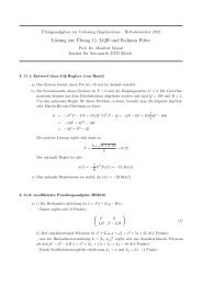
![Convex Optimization: [0.5ex] from Real-Time ... - ETH Zürich](https://img.yumpu.com/18678007/1/190x143/convex-optimization-05ex-from-real-time-eth-zurich.jpg?quality=85)