A Software Defined Radio for the Masses, Part 3

More documents

Recommendations

Info

ate). Since we sample the RF signal in quadrature, the sampling rate is effectively doubled (44,100 Hz times two channels yields an 88,200-Hz effective sampling rate). This means that the output spectrum of the FFT will be twice that of a single sampled channel. In our case, the total output bandwidth of the FFT will be 10.7666 Hz times 4096 or 44,100 Hz. Since most sound cards roll off near 20 kHz, we are probably limited to a total bandwidth of approximately 40 kHz. Fig 5 shows the DLL calls to the Intel library for the FFT and subsequent conversion of the signal vectors from the Cartesian coordinate system to the Polar coordinate system. The nspzrFftNip routine takes the time domain RealIn() and ImagIn() vectors and converts them into frequency domain RealOut() and ImagOut() vectors. The order of the FFT is computed in the routine that calculates the filter coefficients as will be discussed later. NSP_Forw is a constant that tells the routine to perform the forward FFT conversion. In the Cartesian system the signal is represented by the magnitudes of two vectors, one on the Real or x plane and one on the Imaginary or y plane. These vectors may be converted to a single vector with a magnitude (M) and a phase angle (P) in the polar system. Depending on the specific DSP algorithm we wish to perform, one coordinate system or the other may be more efficient. I use the polar coordinate system for most of the signal processing in this example. The nspdbrCartToPolar routine converts the output of the FFT to a polar vector consisting of the magnitudes in M() and the phase values in P(). This function simultaneously performs Eqs 3 and 4 in Part 1 of this article series. Offset Baseband IF Conversion to Zero Hertz My original software centered the RF carrier frequency at bin 0 (0 Hz). With this implementation, one can display (and hear) the entire 44-kHz 4 Nov/Dec 2002 spectrum in real time. One of the problems encountered with direct-conversion or zero-IF receivers is that noise increases substantially near 0 Hz. This is caused by several mechanisms: 1/f noise in the active components, 60/120-Hz noise from the ac power lines, microphonic noise caused by mechanical vibration and local-oscillator phase noise. This can be a problem for weak-signal work because most people tune CW signals for a 700-1000 Hz tone. Fortunately, much of this noise disappears above 1 kHz. Given that we have 44 kHz of spectrum to work with, we can offset the digital IF to any frequency within the FFT output range. It is simply a matter of deciding which FFT bin to des- IFShift = True ‘Force to True for the demo ignate as the carrier frequency and then offsetting the local oscillator by the appropriate amount. We then copy the respective bins for the desired sideband so that they are located at 0 Hz for subsequent processing. In the PC SDR, I have chosen to use an offset IF of 11,025 Hz, which is one fourth of the sampling rate, as shown in Fig 6. Fig 7 provides the source code for shifting the offset IF to 0 Hz. The carrier frequency of 11,025 Hz is shifted to bin 0 and the upper sideband is shifted to bins 1 through 1023. The lower sideband is shifted to bins 3072 to 4094. The code allows the IF shift to be enabled or disabled, as is required for transmitting. If IFShift = True Then ‘Shift sidebands from 11.025KHz IF For S = 0 To 1023 If USB Then M(S) = M(S + 1024) ‘Move upper sideband to 0Hz P(S) = P(S + 1024) Else M(S + 3072) = M(S + 1)‘Move lower sideband to 0Hz P(S + 3072) = P(S + 1) End If Next End If Figure 7 –Code for Down Conversion From Offset Baseband IF to 0Hz If SSB = True Then ‘SSB or CW Modes If USB = True Then For S = FFTBins To NFFT - 1 ‘Zero out lower sideband M(S) = 0 Next Else For S = 0 To FFTBins - 1 ‘Zero out upper sideband M(S) = 0 Next End If End If Figure 8 – Sideband Selection Code Fig 9—FFT fast-convolution-filtering block diagram. The filter impulse-response coefficients are first converted to the frequency domain using the FFT and stored for repeated use by the filter routine. Each signal block is transformed by the FFT and subsequently multiplied by the filter frequency-response magnitudes. The resulting filtered signal is transformed back into the time domain using the inverse FFT. The Overlap/Add routine corrects the signal for circular convolution.
Selecting the Sideband So how do we select sideband? We store zeros in the bins we don’t want to hear. How simple is that? If it were possible to have perfect analog amplitude and phase balance on the sampled I and Q input signals, we would have infinite sideband suppression. Since that is not possible, any imbalance will show up as an image in the passband of the receiver. Fortunately, these imbalances can be corrected through DSP code either in the time domain before the FFT or in the frequency domain after the FFT. These techniques are beyond the scope of this discussion, but I may cover them in a future article. My prototype using INA103 instrumentation amplifiers achieves approximately 40 dB of opposite sideband rejection without correction in software. The code for zeroing the opposite sideband is provided in Fig 8. The lower sideband is located in the highnumbered bins and the upper sideband is located in the low-numbered bins. To save time, I only zero the number of bins contained in the FFTBins variable. FFT Fast-Convolution Filtering Magic Every DSP text I have read on single-sideband modulation and demodulation describes the IF sampling approach. In this method, the A/D converter samples the signal at an IF such as 40 kHz. The signal is then quadrature down-converted in software to baseband and filtered using finite impulse response (FIR) 9 filters. Such as system was described in Doug Smith’s QEX article called, “Signals, Samples, and Stuff: A DSP Tutorial (Part 1).” 10 With this approach, all processing is done in the time domain. For the PC SDR, I chose to use a very different approach called FFT fast-convolution filtering (also called FFT convolution) that performs all filtering functions in the frequency domain. 11 An FIR filter performs convolution of an input signal with a filter impulse response in the time domain. Convolution is the mathematical means of combining two signals (for example, an input signal and a filter impulse response) to form a third signal (the filtered output signal). 12 The time-domain approach works very well for a small number of filter taps. What if we want to build a very-highperformance filter with 1024 or more taps? The processing overhead of the FIR filter may become prohibitive. 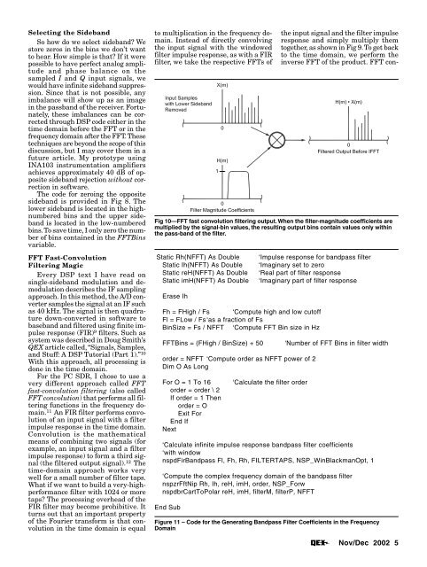It turns out that an important property of the Fourier transform is that convolution in the time domain is equal to multiplication in the frequency domain. Instead of directly convolving the input signal with the windowed filter impulse response, as with a FIR filter, we take the respective FFTs of Fig 10—FFT fast convolution filtering output. When the filter-magnitude coefficients are multiplied by the signal-bin values, the resulting output bins contain values only within the pass-band of the filter. Static Rh(NFFT) As Double ‘Impulse response for bandpass filter Static Ih(NFFT) As Double ‘Imaginary set to zero Static reH(NFFT) As Double ‘Real part of filter response Static imH(NFFT) As Double ‘Imaginary part of filter response Erase Ih Fh = FHigh / Fs ‘Compute high and low cutoff Fl = FLow / Fs‘as a fraction of Fs BinSize = Fs / NFFT ‘Compute FFT Bin size in Hz FFTBins = (FHigh / BinSize) + 50 ‘Number of FFT Bins in filter width order = NFFT ‘Compute order as NFFT power of 2 Dim O As Long For O = 1 To 16 ‘Calculate the filter order order = order \ 2 If order = 1 Then order = O Exit For End If Next ‘Calculate infinite impulse response bandpass filter coefficients ‘with window nspdFirBandpass Fl, Fh, Rh, FILTERTAPS, NSP_WinBlackmanOpt, 1 ‘Compute the complex frequency domain of the bandpass filter nspzrFftNip Rh, Ih, reH, imH, order, NSP_Forw nspdbrCartToPolar reH, imH, filterM, filterP, NFFT End Sub the input signal and the filter impulse response and simply multiply them together, as shown in Fig 9. To get back to the time domain, we perform the inverse FFT of the product. FFT con- Figure 11 – Code for the Generating Bandpass Filter Coefficients in the Frequency Domain Nov/Dec 2002 5
Page 1 and 2: 8900 Marybank Dr Austin, TX 78750 A
Page 3: Signal Processing Library 4 to be l
Page 7 and 8: only have to calculate the filter r
Page 9 and 10: occurs on a 1-ms linear slope. To d

A Software Defined Radio for the Masses, Part 3

Create successful ePaper yourself

Delete template?

Save as template?