2. Mean velocity profiles

2. STRUCTURE OF A TURBULENT BOUNDARY LAYER SPRING 2009
2.1 Shear stress and friction velocity
2.2 Length and velocity scales
2.3 Inner layer
2.4 Outer layer
2.5 Overlap layer – the log law
2.6 Viscous sublayer
2.7 Limits of the various regions
2.8 Velocity-defect layer: Coles’ Law of the Wake
2.9 Effect of roughness
Examples
The analysis is applicable to a flat-plate boundary layer or fully-developed pipe or channel
flow. First consider smooth walls.
2.1 Shear Stress and Friction Velocity
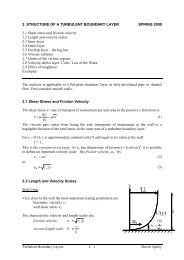
The shear stress (= rate of transport of momentum per unit area in the positive y direction) is
∂U
= − uv
(1)
∂y
The viscous part varies from being the sole transporter of momentum at the wall to a
negligible fraction of the total stress in the outer part of a turbulent boundary layer.
For y < 0.1 , is approximately constant (why?) and equal to its value at the wall:
≈
w
This is the constant-stress layer. As w has dimensions of [density] × [velocity] 2 2¡
, it is possible
to define an important velocity scale – the friction velocity, u – by
w = u
(2)
or
u ≡ /
(3)
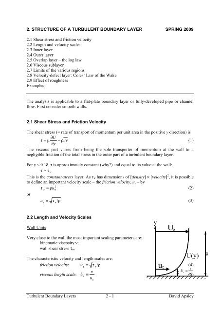
2.2 Length and Velocity Scales
Wall Units
Very close to the wall the most important scaling parameters are:
kinematic viscosity ;
wall shear stress τw.
¢ w
¢ £ ¤ ¥ ¦ § ¨ The characteristic velocity and length scales are:
friction velocity:
viscous length scale:
u ≡ w/
≡
u
uτ
(4)
=
(5) u
Turbulent Boundary Layers 2 - 1 David Apsley
y
Ue
U(y)
δ

From these we can form non-dimensional velocity and height in wall units:
+ U
+ y u y
U ≡ , y ≡ =
u ¡ £
y + is a sort of local Reynolds number. Its value is a measure of the relative importance of
viscous and turbulent transport at different distances from the wall.
Boundary-Layer Units
At large y + the direct effect of viscosity on momentum transport is small and heights can be
specified as a fraction of the boundary-layer depth :
y
= (7)
The quantity
u
Re ≡ ¢ ¢
=
+
is called the friction Reynolds number and is a global parameter of the boundary layer.
Since fully-developed boundary-layer flow is completely specified by U, y, , , and u ,
dimensional analysis (6 variables, 3 independent dimensions) yields a functional relationship
between 6 – 3 = 3 dimensionless groups, conveniently taken as
U y y
= f , )
u
i.e.
+ +
U = f ( y , )
(9) ¢ (£
Almost all boundary-layer analysis is based upon the smooth overlap of the limiting cases –
inner layer ( 0) and outer layer (y + » 1).
2.3 Inner Layer (Prandtl, 1925)
Dimensional parameters U, y, w, , – but not .
dimensionless groups, conveniently taken as ¡
Dimensional analysis (5 parameters, 3 independent dimensions) ⇒ 2 independent
+
U
+
= U / u and y = u¡y
/ .
Then we have the law of the wall:
+ +
U = f w ( y )
(10)
fw is expected to be a universal function; i.e. independent of the external flow.
According to Pope (2000), the inner layer corresponds roughly to y / < 0.1, or the region
over which the shear stress is approximately constant.
Turbulent Boundary Layers 2 - 2 David Apsley
(6)
(8)

2.4 Outer Layer (Von Kármán, 1930)
Dimensional parameters U, y, w, , – but not .
Dimensional analysis (5 parameters, 3 independent dimensions) ⇒ 2 independent
dimensionless groups, conveniently taken as
U e −U
y
,
=
u
Then one has the velocity-defect law:
U e −U
= f o ( )
(11)
u
Unlike fw which is expected to be universal, fo( ) will vary with the particular flow.
¢
2.5 Overlap Layer – the Log Law
As noted by C.B. Millikan (1937) the inner and outer layers can only overlap smoothly if the
overlap-region velocity profile is logarithmic.
Outer layer: U − U = f ( )
+ +
e o
Inner layer:
+ +
U = f w ( y )
Introducing + = u / , so that y + =
+
U (
+
) f ( ) + f (
+
)
e
= o w
+ , and adding:
+ to be the sum of separate functions of and + , fw must
For a function fw of the product
be logarithmic. This can be proved formally by differentiating successively with respect to
each variable, as follows.
Differentiate wrt + :
U
′
(
+
) = 0 +
+ ′
e
f w
Differentiate wrt η:
0 = f ′ (
w
+
) +
(
+
)
f ′
(
+
w
+
w
+
)
+ +
= f ′ ( ) ′′
w y + y f ( y
d + df
w
= ( y )
+
+
dy
dy
)
Hence,
+ df
w
y +
dy
= constant
This constant is conventionally written as 1/ , where (≈ 0.41), is von Kármán’s constant.
+ + = df
w
dy
1
y
which integrates to give
1 +
= ln y + B , B another constant.
f w
Turbulent Boundary Layers 2 - 3 David Apsley

Hence we have the log-law velocity profile:
+ 1 +
U = ln y + B
or, equivalently,
+ 1
U = ln Ey
+
Notes.
(1) There is some variation between sources, but typical values of the constants are
= 0.41 (1/ = 2.44) and B = 5.0 (E = 7.76).
(2) Except in strong adverse pressure gradients (e.g. in a diffuser) the logarithmic velocity
profile is a good approximation across much of the shear layer. This observation turns
out to extremely useful in deriving friction formulae – see Section 3.
(3) In the log law region,
+
∂U
u
y ∂U
+ ∂U
= or = y = constant
+
∂y
y
u ∂y
∂y
This is often used as an alternative starting point for the derivation of the log law. ¢ ¢
2.6 Viscous Sublayer
Very close to the wall, turbulent fluctuations are damped out and the wall shear stress is
almost entirely viscous:
∂U
= w , constant
∂y
which yields a linear velocity profile:
Setting
U
w
=
w
y
= and rearranging,
u 2¡
+ +
U = y
(14)
Experiment shows that the linear viscous sublayer corresponds roughly to y + < 5.
2.7 Limits of the Various Regions
Pope (2000) gives the following rough delimiting y + and y/ values.
Inner layer (roughly y/ < 0.1) – velocity scales on u and y + , but not on .
Outer layer (roughly y + > 50) – the direct effect of viscosity is negligible.
Overlap region - exists at sufficiently high Reynolds number.
In the overlap region the mean-velocity profile must be logarithmic. In fact the log law is a
good approximation beyond the overlap region. Pope suggests:
Turbulent Boundary Layers 2 - 4 David Apsley
(12)
(13)

Viscous sublayer: y + < 5 – linear velocity profile
Buffer layer: 5 < y + < 30
Log law region: y + > 30, y/ < 0.3 – logarithmic velocity profile
2.8 Velocity-Defect Layer: Coles’ Law of the Wake
In the outer layer the velocity profile deviates slightly from the log law, particularly in nonequilibrium
boundary layers with a pressure gradient. Coles (1956) noted that the deviation or
excess velocity above the log law had a wake-like shape relative to the free stream; i.e.
y
U = U + U f ( )
log law
where f is some S-shaped function with f(0) = 0, f(1) = 1; popular forms are
f (
2
) = sin
2
f ( ) = 3
2
− 2
3
Then we have the Coles Law of the Wake:
U
u
1 +
= ln y
2
+ B + f ( y/
)
where the deviation from the log law is quantified by the Coles wake parameter .
Typical values are:
pipe flow or channel flow: = 0
zero-pressure-gradient flat-plate boundary layer: = 0.45
In general, is a function of pressure gradient.
2.9 Effect of Roughness
The seminal experimental work was done by Prandtl’s PhD student Johann Nikuradse, who
measured the friction factor in pipes artificially roughened with densely-packed sand grains
of size ks. The relative roughness ks/D varied from 1/30 to 1/1000.
+
The influence of wall roughness is characterised by k = u k /
+
Hydraulically Smooth: ( k s < 5 ; i.e. less than the viscous sublayer depth)
In this regime roughness has no effect on the friction factor or mean-velocity profile.
+
Fully Rough: ( k s > 70 )
Transfer of momentum to the wall is predominantly by pressure drag on roughness elements,
not viscous stresses, and wall friction becomes essentially independent of Reynolds number
for sufficiently large Re. Dimensional analysis implies
+ 1 y
U = ln + Bk
k
From experimental data, Bk ≈ 8.5.
s
Turbulent Boundary Layers 2 - 5 David Apsley
s
¡s
.
(15)

Transitional Roughness ( 5 < < 70
+
k s )
Both roughness and viscous effects operate.
+
(These k s limits are those of Schlichting. White gives 4 and 60 instead, whilst Cebeci and
Bradshaw’s transition formula below uses 2.25 and 90.)
An all-encompassing mean-velocity profile may be written
+ 1 +
ln
~ +
+ ( ) k B y U
where
~
B
= s
⎧B
⎪
⎨
⎪⎩
B
( k
→
k
1 +
− ln k s
+
s
+
( k s
Suitable interpolation formulae are:
Cebeci and Bradshaw (1977):
→
~ 1 +
B ( 1−
) B + ( B − ln k ) ,
= k
s
Apsley (2007):
~ 1
= B − ln( k
+
B k
s
+ C)
,
0;
hydraulically
smooth)
→ ∞;
fully rough)
⎧ 0 ,
⎪
+
⎪ ⎡ ln( k ⎤
s / 2.
25)
= ⎨ sin⎢
⎥ ,
⎪ ⎣ 2 ln( 90 / 2.
25)
⎦
⎪⎩
1 ,
C = e
( Bk −B
)
> 90
< 90
Turbulent Boundary Layers 2 - 6 David Apsley
k
+
s
+
s
<
2.
25
k
2.
25
(Both authors used slightly different values of B and Bk from those used in these Notes).
In practice, we are often more interested in the resulting friction law (see Section 3). For pipe
flow this is the Colebrook-White formula. The effect of surface roughness depends on its
form as well as its size. The work of Colebrook (1939) and Moody (1944) helped to define
“equivalent sand roughness” for many commercial pipe materials.
Geophysical Flows
Perhaps the ultimate in rough-wall boundary layers is the atmospheric boundary layer. In this
case the mean velocity profile is typically written (with the meteorological convention of z
for a vertical coordinate):
u z
U = ln( )
(16)
z0
z0 is called the roughness length and comparison with the above formulae, fitting all
constants inside the natural logarithm and taking Bk = 8.5, gives z0 ≈ k s / 30 . For typical rural
conditions z0 has a value of about 0.1 m.
¡
< k
+
s

Examples
Question 1.
Consider airflow at 10 m s –1 over a flat plate. If the friction Reynolds number is 1200,
calculate (a) the friction velocity; (b) the wall shear stress; (c) the depth of the boundary
layer. Assume a Coles wake parameter = 0.45.
Question 2.
Wind velocities over open fields were measured as 5.89 m s –1 and 8.83 m s –1 at heights of
2 m and 10 m respectively. Use this data to estimate: (a) the roughness length z0; (b) the
friction velocity u ; (c) the velocity at height 25 m; (d) the average velocity over a depth of
25 m.
Question 3. (From White, 1994)
J. Laufer’s (1954) pipe-flow experiments gave the following data at ReD ≈ 5×10 5
r/R 0.0 0.102 0.206 0.412 0.617 0.784 0.846 0.907 0.963
U/U0 1.0 0.997 0.988 0.959 0.908 0.847 0.818 0.771 0.690
where U0 is the centreline velocity. Find the best-fit power-law profile of the form
U
U 0
y 1/
n
= ( )
R
where y = R – r is the distance from the wall.
Answers
(1) (a) u = 0.41 m s –1
(b) w = 0.20 N m –2
(c) = 44 mm
(2) (a) z0 = 0.080 m
(b) u = 0.75 m s –1
(c) U(z = 25 m) = 10.5 m s –1
(d) Uav = 8.7 m s –1
(3) n = 9
Turbulent Boundary Layers 2 - 7 David Apsley