2. Mean velocity profiles

Transitional Roughness ( 5 < < 70
+
k s )
Both roughness and viscous effects operate.
+
(These k s limits are those of Schlichting. White gives 4 and 60 instead, whilst Cebeci and
Bradshaw’s transition formula below uses 2.25 and 90.)
An all-encompassing mean-velocity profile may be written
+ 1 +
ln
~ +
+ ( ) k B y U
where
~
B
= s
⎧B
⎪
⎨
⎪⎩
B
( k
→
k
1 +
− ln k s
+
s
+
( k s
Suitable interpolation formulae are:
Cebeci and Bradshaw (1977):
→
~ 1 +
B ( 1−
) B + ( B − ln k ) ,
= k
s
Apsley (2007):
~ 1
= B − ln( k
+
B k
s
+ C)
,
0;
hydraulically
smooth)
→ ∞;
fully rough)
⎧ 0 ,
⎪
+
⎪ ⎡ ln( k ⎤
s / 2.
25)
= ⎨ sin⎢
⎥ ,
⎪ ⎣ 2 ln( 90 / 2.
25)
⎦
⎪⎩
1 ,
C = e
( Bk −B
)
> 90
< 90
Turbulent Boundary Layers 2 - 6 David Apsley
k
+
s
+
s
<
2.
25
k
2.
25
(Both authors used slightly different values of B and Bk from those used in these Notes).
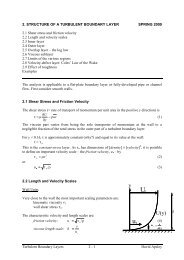
In practice, we are often more interested in the resulting friction law (see Section 3). For pipe
flow this is the Colebrook-White formula. The effect of surface roughness depends on its
form as well as its size. The work of Colebrook (1939) and Moody (1944) helped to define
“equivalent sand roughness” for many commercial pipe materials.
Geophysical Flows
Perhaps the ultimate in rough-wall boundary layers is the atmospheric boundary layer. In this
case the mean velocity profile is typically written (with the meteorological convention of z
for a vertical coordinate):
u z
U = ln( )
(16)
z0
z0 is called the roughness length and comparison with the above formulae, fitting all
constants inside the natural logarithm and taking Bk = 8.5, gives z0 ≈ k s / 30 . For typical rural
conditions z0 has a value of about 0.1 m.
¡
< k
+
s