WAVES AND VIBRATIONS IN INHOMOGENEOUS STRUCTURES ...

Normalized amplitude
1
0.9
0.8
0.7
0.6
0.5
0.4
0.3
0.2
0.1
0
0 20 40 60 80 100
Frequency (rad/s)
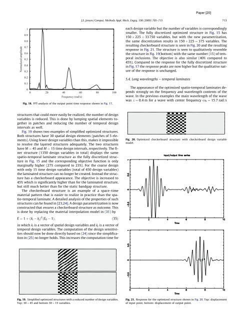
Fig. 18. FFT-analysis of the output point time response shown in Fig. 17.
structures that could more easily be realized, the number of design
variables is reduced. This is done by lumping spatial elements together
in patches and reducing the number of temporal design
intervals as well.
Fig. 19 shows two examples of simplified optimized structures.
Both structures have 30 spatial design elements (patches of 5 elements).
Using fewer design variables than this, makes it impossible
to resolve the layered structures adequately. The two structures
have M ¼ 45 and M ¼ 15 time design intervals, respectively. The finer
structure (1350 design variables in total) displays the same
spatio-temporal laminate structure as the fully discretized structure
in Fig. 15 and the corresponding objective function is only
marginally higher (27% compared to 23%). For the coarse design
with only 15 time design variables (total of 450 design variables)
the laminated structure can no longer be created. Instead the structure
has a checkerboard appearance. The objective is increased to
45% which is significantly higher than for the laminated structure,
but still much better than for the static bandgap structure.
The checkerboard structure is an example of a space–time
material pattern that is easier to realize in practice than the spatio-temporal
laminate. A detailed analysis of the properties of such
structures can be found in [23,24]. A design parametrization is now
constructed that ensures a checkerboard structure as outcome. This
is done by replacing the material interpolation model in (31) by
E ¼ 1 þð~xi ~xjÞ 2 ðE0 1Þ; ð35Þ
in which ~xi is a vector of spatial design variables and ~xj is a vector of
temporal design variables. The computation of the design sensitivities
should now be done directly based on (24) since the simplification
in (25) no longer holds. This increases the computation time for
Fig. 19. Simplified optimized structures with a reduced number of design variables.
Top: 30 45 and bottom 30 15 variables.
J.S. Jensen / Comput. Methods Appl. Mech. Engrg. 198 (2009) 705–715 713
each design variable but the number of variables is correspondingly
smaller. The fully discretized optimized structure in Fig. 15 has
150 225 ¼ 33750 variables, but with the new parametrization,
the same discretization results in 150 þ 225 ¼ 375 variables. The
resulting checkerboard structure is seen in Fig. 20 and the resulting
response in Fig. 21. The structure is seen to qualitatively resemble
the structure in Fig. 19(bottom) with the same number (15) of temporal
inclusions. The objective is also similar (40% compared to
45%). Compared to the response for the fully discretized structure
in Fig. 17 the response peaks are now higher but the qualitative nature
of the response is unchanged.
5.4. Long wavelengths – temporal laminates
The appearance of the optimized spatio-temporal laminates depends
strongly on the frequency and wavelength contents of the
wave. In the previous examples the main wavelength of the wave
was k ¼ 0:4 m for a wave with center frequency x0 ¼ 15:7 rad=s
Fig. 20. Optimized checkerboard structure with checkerboard design variable
model.
Fig. 21. Response for the optimized structure shown in Fig. 20. Top: displacement
of input point, bottom: displacement of output point.