WAVES AND VIBRATIONS IN INHOMOGENEOUS STRUCTURES ...

710 J.S. Jensen / Comput. Methods Appl. Mech. Engrg. 198 (2009) 705–715
and further require that the initial response at t ¼ 0 is independent
of the design such that
u 0j
i ð0Þ ¼ _u 0j
i ð0Þ ¼0: ð19Þ
Inserting (17)–(19) into (16) yields
U 0j
i ¼
Z T
0
€k T
j M _ k T
j
@c
C þ kT
j K þ
@u u0j
i
þ kT
j K0j
i
u þ c0j
i
dt: ð20Þ
The arbitrary adjoint vectors kj are now chosen so that the first
parenthesis in (20) vanishes
€k T
j M _ k T
j
@c
C þ kT
j K þ ¼ 0; ð21Þ
@u
which, after transposing, can be rewritten as
M T€ kj C T _ kj þ K T kj ¼
@c
@u
T
: ð22Þ
As appears from (22) all adjoint equations are identical since the
r.h.s. does not depend on j. Thus only one equation needs to be
solved and the substitution kj ¼ k is made.
Eq. (22) is conveniently rewritten by introducing the new time
variable s ¼ T t
M T€ k þ C T _ k þ K T k ¼
@c
@u
T
T s
: ð23Þ
Thus, with symmetric matrices, M T ¼ M, C T ¼ C, K T ¼ K, the l.h.s. of
(23) is identical to that of the original model equation (1), the only
difference being the new adjoint load that appears on the r.h.s.
However, it should be noted that the two equations cannot be
solved simultaneously due the r.h.s. of (23) that requires an evaluation
of @c=@u at time T s.
When k fulfills (23) the expression for the sensitivities reduces
to
U 0j
i ¼
Z T
0
ðk T ðT tÞK 0j
i u þ c0j
i Þdt; ð24Þ
in which it is specified that k should be evaluated at s ¼ T t. The
term K 0j
i denotes the derivative of the stiffness matrix w.r.t. the i0 th
element design variable in the j 0 th time interval, thus
K 0j
i ¼ 0 for t < T j
and t > Tþ
j ; ð25Þ
in which T j and T þ
j is the start and finish point for the j 0 th time
interval. Thus,
U 0j
i ¼
Z T
0
c 0j
i dt þ
Z T þ
j
T j
k T ðT tÞðKjÞ 0
iudt; ð26Þ
in which Kj is the stiffness matrix in the j 0 th time interval.
It is assumed that the stiffness matrix KðtÞ can be written in the
following form:
KðtÞ ¼ XN
i¼1
EiðtÞK i ; ð27Þ
in which EiðtÞ is the element-wise and time dependent Young’s
modulus and K i is a local element matrix. With the temporal discretization
of the design space
Kj ¼ XN
i¼1
such that
ðKjÞ 0
i
¼ dE
Eðx j
i ÞKi
dx j K
i
i
and the expression for the sensitivities becomes
ð28Þ
ð29Þ
U 0j
i ¼
Z T
0
c 0j
i
dt þ dE
dx j
i
Z T þ
j
T j
in which k i and u i are local element vectors.
ðk i Þ T ðT tÞK i u i dt; ð30Þ
4.1. Material interpolation and optimization algorithm
The material properties in the design elements are interpolated
linearly based on the design variables. Thus, the stiffness of element
i in time interval j is
E ¼ 1 þ x j
i ðE0 1Þ; ð31Þ
in which the stiffness of the ‘‘background” material is set to unity as
in the numerical examples in Section 3. Thus, the expression in (30)
can be further reduced to
U 0j
i ¼
Z T
0
c 0j
i dt þðE0 1Þ
Z T þ
j
T j
ðk i Þ T ðT tÞK i u i dt: ð32Þ
Thus, sensitivities w.r.t. all design variables are obtained by solving
the additional problem (23) followed, for each variable, by the integration
in (32) which is carried out numerically. If the objective
function does not depend explicitly on the design variables the first
integral in (32) vanishes and no extra computational effort is required
to handle the space–time design variables compared to the
case of static design variables. However, the need to store u and k
at each time step can be a significant computational burden, but
has been solved previously for a 3D problem in [28].
Optimized space–time structures are generated on the basis of
the computed sensitivities by using a gradient-based algorithm.
A mathematical programming software, MMA [32], is used to obtain
the design updates and forward analysis, sensitivity analysis
and design updates are continued in an iterative fashion until the
design converges. See, e.g. [4] for a detailed description of the iterative
optimization algorithm.
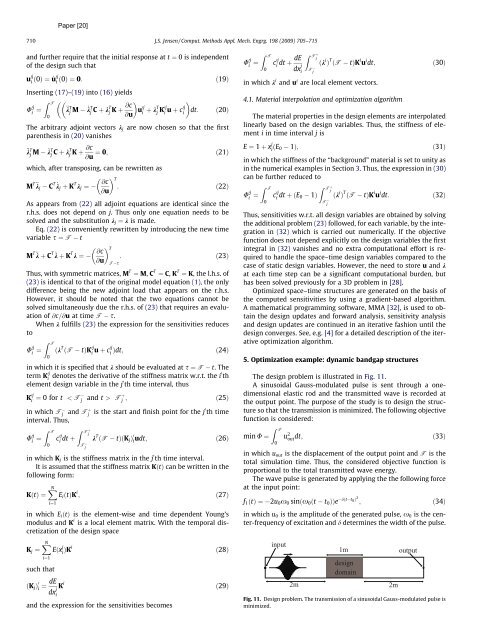
5. Optimization example: dynamic bandgap structures
The design problem is illustrated in Fig. 11.
A sinusoidal Gauss-modulated pulse is sent through a onedimensional
elastic rod and the transmitted wave is recorded at
the output point. The purpose of the study is to design the structure
so that the transmission is minimized. The following objective
function is considered:
min U ¼
Z T
0
u 2
outdt; ð33Þ
in which uout is the displacement of the output point and T is the
total simulation time. Thus, the considered objective function is
proportional to the total transmitted wave energy.
The wave pulse is generated by applying the the following force
at the input point:
f1ðtÞ ¼ 2u0x0 sinðx0ðt t0ÞÞe dðt t 0Þ 2
; ð34Þ
in which u0 is the amplitude of the generated pulse, x0 is the center-frequency
of excitation and d determines the width of the pulse.
input
1m
design
domain
2m 2m
output
Fig. 11. Design problem. The transmission of a sinusoidal Gauss-modulated pulse is
minimized.