WAVES AND VIBRATIONS IN INHOMOGENEOUS STRUCTURES ...

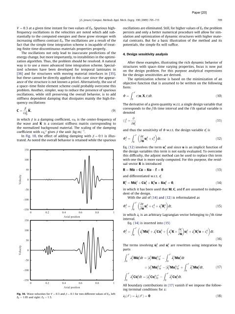
V ¼ 0:3 at a given time instant for two values of E0. Spurious highfrequency
oscillations in the velocities are noted which add substantially
to the computed energies and these grow stronger with
increasing stiffness contrast E0. The oscillations are a result of the
fact that the simple time integration scheme is incapable of treating
finite time-discontinuous materials properties properly.
The oscillations not only lead to inaccurate predictions of the
energy change, but more importantly, to instabilities in the optimization
algorithm. Thus, the problem should be resolved. A natural
way is to use a more advanced time integration scheme. Specialized
schemes have been developed for temporal laminates in
[36] and for structures with moving material interfaces in [35],
but these cannot be directly applied in this case since the appearance
of the structure is not known a priori. Alternatively, the use of
a space–time finite element scheme could probably overcome this
problem. Another, simpler, way to reduce the presence of spurious
oscillations, while still preserving the overall behavior, is to add
stiffness dependent damping that dissipates mainly the high-frequency
oscillations
C ¼ b
x2 eK; ð9Þ
0
in which b is a damping coefficient, x0 is the center-frequency of
the wave and e K is a constant stiffness matrix corresponding to
the normalized background material. The scaling of the damping
coefficient with x 2
0 gives b the unit ðkg mÞ 1 .
In Fig. 10, the effect of adding damping with b ¼ 0:1 is illustrated.
As noted the overall behavior is retained while the spurious
Velocity
Velocity
150
100
50
0
-50
-100
-150
0 0.2 0.4 0.6 0.8 1
Axial position
150
100
50
0
-50
-100
-150
0 0.2 0.4 0.6 0.8 1
Axial position
Fig. 10. Wave velocities for V ¼ 0:3 and b ¼ 0:1 for two different values of E0, left:
E0 ¼ 1:05 and right: E0 ¼ 1:5.
J.S. Jensen / Comput. Methods Appl. Mech. Engrg. 198 (2009) 705–715 709
oscillations are eliminated. Still, for higher values of E0 the problem
persists and only a better numerical procedure will allow for simulation
and optimization of dynamic structures with higher material
contrasts. But for a basic illustration of the method and its
potentials, the simple fix will suffice.
4. Design sensitivity analysis
After these examples, illustrating the rich dynamic behavior of
structures with space–time varying properties, focus is now put
on the design problem. For this purpose analytical expressions
for the design sensitivities are derived.
The optimization scheme is based on the minimization of an
objective function that is assumed to be written on the following
form:
U ¼
Z T
0
cðu; X; tÞdt: ð10Þ
The derivative of a given quantity w.r.t. a single design variable that
corresponds to the j 0 th time interval and the i 0 th spatial variable is
denoted
ðÞ 0j
i
¼ @
@x j
i
and thus the sensitivity of U w.r.t. the design variable x j
i is
U 0j
i ¼
Z T
0
@c
@u u0j
i
þ c0j
i
ð11Þ
dt: ð12Þ
Eq. (12) involves the term u 0j
i and since u is an implicit function of
the design variables this term is not easily evaluated. To overcome
this difficulty, the adjoint method can be used to replace this term
with one that is more easily computed. For this purpose, the residual
vector R is introduced
R ¼ M€u þ C _u þ Ku f ¼ 0 ð13Þ
and differentiated w.r.t. x j
i
R 0j 0j
i ¼ M€u
i þ C _u 0j
i
þ K0j
i u þ Ku0j
i ¼ 0; ð14Þ
in which it has been used that M, C, and f are assumed to independent
of the design.
With the aid of (14) and (12) is reformulated as
U 0j
i ¼
Z T
0
@c
@u u0j
i
þ c0j
i þ kT
j R0j
i
dt; ð15Þ
in which kj is an arbitrary Lagrangian vector belonging to j 0 th time
interval.
U 0j
i ¼
Eq. (14) is inserted into (15)
Z T
0
k T
j
0j
M€u i þ kT
j C _u 0j
i
@c
þ kT
j K þ
@u u0j
i
þ kT
j K0j
i
u þ c0j
i dt:
ð16Þ
The terms involving €u 0j
i and _u 0j
i are rewritten using integration by
parts
Z T
0
k T
j
Z T
k
0
T
j C _u 0j
i
0j
M€u i dt ¼½kT j M _u 0j
i ŠT
0
dt ¼½kT
¼½k T
j M _u 0j
i ŠT
0
j Cu0j
i ŠT
0
Z T
0
_k T
j M _u 0j
i dt
½ _ k T
j Mu0j
i ŠT
0 þ
Z T
0
_k T
j Cu0j
i dt:
Z T
0
€k T
j Mu0j
i dt;
ð17Þ
All boundary contributions in (17) vanish if we impose the following
terminal conditions for k:
kjðTÞ ¼ _ kjðTÞ ¼0 ð18Þ