

WAVES AND VIBRATIONS IN INHOMOGENEOUS STRUCTURES ...
WAVES AND VIBRATIONS IN INHOMOGENEOUS STRUCTURES ...
WAVES AND VIBRATIONS IN INHOMOGENEOUS STRUCTURES ...

You also want an ePaper? Increase the reach of your titles
YUMPU automatically turns print PDFs into web optimized ePapers that Google loves.
1194 J. Opt. Soc. Am. B/Vol. 22, No. 6/June 2005 J. S. Jensen and O. Sigmund<br />
Hˆ e = rmin − distk,e, e Ddistk,e rmin, k =1, ..., N D . 16<br />
Thus the filtered sensitivities is a modification of the<br />
original sensitivities based on a weighted average of the<br />
sensitivities in neighboring elements within a fixed range<br />
(specified by r min). In the examples shown, we have used<br />
r min=2.5 times the element size.<br />
C. Continuation Method and Penalization<br />
The solution of the optimization problem turns out to be<br />
strongly nonunique, which results in multiple local<br />
maxima. Some of these are based on local resonance effects<br />
that lead to a poor performance away from the target<br />
frequency and to strong out-of-plane scattering and,<br />
consequently, to poor transmission for a real threedimensional<br />
structure. A way to reduce the chance of ending<br />
up in such a maximum is to apply a continuation<br />
method in which we attempt to convexify the object function<br />
by changing the original problem into a smoother<br />
one. After a converged design is obtained for the smooth<br />
problem, we gradually change the problem back into its<br />
original form during a continued optimization procedure.<br />
As shown for phononic bandgap structures, 18 the presence<br />
of strong damping smoothes the dynamic response<br />
considerably, and in Ref. 13 this was used with advantage<br />
to avoid undesired local extrema in the optimization of<br />
these structures.<br />
Similar to the case of phononics (elastic waves), we<br />
here add an artificial damping term C art to the model:<br />
C = C abs + C art, 17<br />
where C abs is the damping matrix stemming from the absorbing<br />
boundaries. We let the extra damping matrix be<br />
proportional to the mass matrix, such that<br />
C art = M, 18<br />
where is a real and positive constant. In a typical optimization<br />
procedure we start out with strong damping,<br />
say, =0.1, and then gradually decrease until the performance<br />
of the structure no longer can be improved.<br />
Even when avoiding the pitfall of resonance-based local<br />
maxima, we may still end up with an unfeasible design<br />
with elements that have nondiscrete design variables x e,<br />
i.e., values other than strictly 0 or 1. For other applications<br />
of topology optimization, various penalization methods<br />
have been developed to avoid this problem. For<br />
bandgap-type problems, the need for penalization appears<br />
to be small 13 in that the highest possible material contrast<br />
is favorable for maximum wave reflection. However,<br />
if the problem is not strictly of the reflection type, we may<br />
end up with some gray elements.<br />
Here we propose a new scheme inspired by an explicit<br />
penalization scheme introduced in Ref. 19. Instead of adding<br />
a penalization term directly to the objective, we use<br />
an implicit variant by introducing the penalty as an extra<br />
damping term for elements in D:<br />
e<br />
Cpen =4xe1−xeMe , e D, 19<br />
thereby causing elements with 0x e1 to induce an energy<br />
loss and hence be expensive for the objective function.<br />
The penalization scheme is typically employed when<br />
a converged design is obtained and gray elements have<br />
appeared. Then is gradually increased from, e.g., <br />
=0.01 until the gray elements vanish. However, if a lot of<br />
gray elements appear in the design, it can be beneficial to<br />
have a nonzero throughout the optimization procedure.<br />
In the following we call the pamping coefficient as an acronym<br />
for penalization damping.<br />
D. Algorithm<br />
The optimization algorithm is outlined in the following:<br />
1. Set up a finite-element model and choose an appropriate<br />
design domain D and target frequency .<br />
2. Choose an initial design, i.e., distribution of xe in D, and initial values of artificial damping, e.g., =0.1.<br />
3. Compute the elementwise material coefficients Ae and Be. 4. Solve system equations and compute objective func-<br />
ˆ<br />
tion J and filtered design sensitivities dJ/dxe.<br />
5. Update design with the mathematical programming<br />
tool, the Method of Moving Asymptotes. 17<br />
6. Repeat steps (3)–(5) until design convergence is<br />
maxx new−x e, where is a small positive constant.<br />
7. Decrease artificial damping, e.g., new=/2.<br />
8. Repeat steps (3)–(7) until the performance is no<br />
longer improved.<br />
9. If gray elements appear in the design, repeat steps<br />
(3)–(5) with increasing values of , starting from, e.g., <br />
=0.01. Alternatively, carry out the whole optimization<br />
procedure with a nonzero .<br />
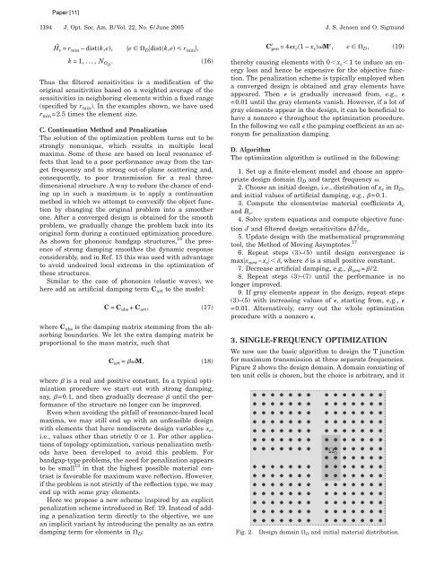
3. S<strong>IN</strong>GLE-FREQUENCY OPTIMIZATION<br />
We now use the basic algorithm to design the T junction<br />
for maximum transmission at three separate frequencies.<br />
Figure 2 shows the design domain. A domain consisting of<br />
ten unit cells is chosen, but the choice is arbitrary, and it<br />
Fig. 2. Design domain D and initial material distribution.


