- Page 1 and 2:
WAVES AND VIBRATIONS IN INHOMOGENEO
- Page 3:
Denne afhandling er af Danmarks Tek
- Page 7 and 8:
List of Thesis Papers [1] J. S. Jen
- Page 9 and 10:
Contents Preface i List of Thesis P
- Page 11 and 12:
Chapter 1 Introduction This thesis
- Page 13 and 14:
eplacemen Phononic and photonic ban
- Page 15 and 16:
Optimal material distribution - top
- Page 17 and 18:
Chapter 2 The bandgap phenomenon In
- Page 19 and 20:
2.1 Band diagram and forced vibrati
- Page 21 and 22:
2.3 Experimental demonstration 11 F
- Page 23 and 24:
y 2.5 Nonlinearities 13 Response in
- Page 25 and 26:
Relations to recent work 15 Amplitu
- Page 27 and 28:
Chapter 3 Bandgap structures as opt
- Page 29 and 30:
3.1 Vibration-quenching structures
- Page 31 and 32:
3.2 Maximizing wave reflection 21 d
- Page 33 and 34:
3.4 Maximizing wave dissipation 23
- Page 35 and 36:
3.4 Maximizing wave dissipation 25
- Page 37 and 38:
3.5 Plate structures 27 a) b) Figur
- Page 39 and 40:
3.6 Acoustic design 29 design domai
- Page 41 and 42:
Chapter 4 Optimization of photonic
- Page 43 and 44:
4.1 Waveguide bends and junctions 3
- Page 45 and 46:
4.2 Photonic crystal building block
- Page 47 and 48:
4.2 Photonic crystal building block
- Page 49 and 50:
4.4 Ridge waveguides 39 w ε =1 ?
- Page 51 and 52:
Relations to recent work 41 wave in
- Page 53 and 54:
Chapter 5 Advanced optimization pro
- Page 55 and 56:
5.1 Padé approximants 45 h 2h A f
- Page 57 and 58:
5.3 Space-time topology optimizatio
- Page 59 and 60:
5.3 Space-time topology optimizatio
- Page 61 and 62:
Relations to recent work 51 Figure
- Page 63 and 64:
Chapter 6 Conclusions In the first
- Page 65 and 66:
References K. Asakawa, Y. Sugimoto,
- Page 67 and 68:
References 57 W. R. Frei, D. A. Tor
- Page 69 and 70:
References 59 F. Maestre, A. Münch
- Page 71 and 72:
References 61 O. Sigmund, J. S. Jen
- Page 73 and 74:
References 63 X. M. Zhou and G. K.
- Page 75 and 76:
Dansk resumé 65 i strukturen. En r
- Page 77 and 78:
1054 ARTICLE IN PRESS J.S. Jensen /
- Page 79 and 80:
1056 ARTICLE IN PRESS J.S. Jensen /
- Page 81 and 82:
1058 fundamental eigenfrequency o
- Page 83 and 84:
1060 ðo 2 y;j;k ARTICLE IN PRESS J
- Page 85 and 86:
1062 local resonator and splits up
- Page 87 and 88:
1064 3.1. Model equations A finite
- Page 89 and 90:
1066 FRF (dB) 150 100 50 0 -50 -100
- Page 91 and 92:
1068 3.3. Example 2: a 2-D waveguid
- Page 93 and 94:
1070 ARTICLE IN PRESS J.S. Jensen /
- Page 95 and 96:
1072 ARTICLE IN PRESS J.S. Jensen /
- Page 97 and 98:
1074 ARTICLE IN PRESS J.S. Jensen /
- Page 99 and 100:
1076 ARTICLE IN PRESS J.S. Jensen /
- Page 101 and 102:
1078 ARTICLE IN PRESS J.S. Jensen /
- Page 103 and 104:
wave-guiding properties show promis
- Page 105 and 106:
(a) (b) Acceleration response (dB)
- Page 107 and 108:
B.S. Lazarov, J.S. Jensen / Interna
- Page 109 and 110:
ω/κ ω/κ 1.5 1.4 1.3 1.2 1.1 1 0
- Page 111 and 112:
[B 2000 ] [B 2000 ] [B 2000 ] 0.25
- Page 113 and 114:
[B 400 ] 0.25 0.2 0.15 0.1 0.05 B.S
- Page 115 and 116:
1002 (a) (c) (e) 0. Sigmund and J.
- Page 117 and 118:
1004 O. Sigmund and J. S. Jensen wh
- Page 119 and 120:
1006 (a) - - - - - - _ - - - - I I
- Page 121 and 122:
1008 O. Sigmund and J. S. Jensen we
- Page 123 and 124:
1010 O. Sigmund and J. S. Jensen Th
- Page 125 and 126:
1012 (a) (b) O. Sigmund and J. S. J
- Page 127 and 128:
1014 . ct . _ a) Q^ s^c "3
- Page 129 and 130:
1016 O. Sigmund and J. S. Jensen (a
- Page 131 and 132:
1018 O. Sigmund and J. S. Jensen 4.
- Page 134 and 135:
Z. Kristallogr. 220 (2005) 895-905
- Page 136 and 137:
Inverse design of phononic crystals
- Page 138 and 139:
Inverse design of phononic crystals
- Page 140 and 141:
Inverse design of phononic crystals
- Page 142 and 143:
Inverse design of phononic crystals
- Page 144:
Inverse design of phononic crystals
- Page 147 and 148:
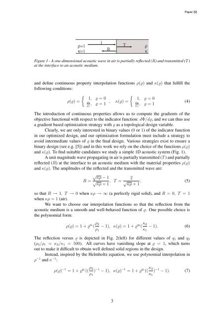
320 Optimization of the dissipation
- Page 149 and 150: 322 The reflection of the wave is f
- Page 151 and 152: 324 which averaged over a wave peri
- Page 153 and 154: 326 where the modified stress compo
- Page 155 and 156: 328 optimization algorithm is enhan
- Page 157 and 158: 330 reflectance are also seen (Fig.
- Page 159 and 160: 332 It should be emphasized that ot
- Page 161 and 162: 334 b Dissipation, D c Dissipation,
- Page 163 and 164: 336 7.2. Three-phase design ARTICLE
- Page 165 and 166: 338 ARTICLE IN PRESS J.S. Jensen /
- Page 167 and 168: 340 ARTICLE IN PRESS J.S. Jensen /
- Page 169 and 170: 968 ARTICLE IN PRESS J.S. Jensen, N
- Page 171 and 172: 970 To solve the wave equation with
- Page 173 and 174: 972 In the following section, we sh
- Page 175 and 176: 974 Design variable, t Design varia
- Page 177 and 178: 976 Eigenvalue ratio, ω n+1 2 /ωn
- Page 179 and 180: 978 to a design parameter te are gi
- Page 181 and 182: 980 ARTICLE IN PRESS J.S. Jensen, N
- Page 183 and 184: 982 respect to the higher bound C1
- Page 185 and 186: 984 instead vary the value of b. Th
- Page 187 and 188: 986 References ARTICLE IN PRESS J.S
- Page 189 and 190: a thick solid was considered. A few
- Page 191 and 192: The above expressions provide insta
- Page 193 and 194: In all the examples shown a density
- Page 195 and 196: domain. To the very left the passiv
- Page 197 and 198: Jensen JS, Sigmund O (2005) Topolog
- Page 199: paper extends on this work. For an
- Page 203 and 204: objective 1 0.9 0.8 0.7 0.6 0.5 0.4
- Page 205 and 206: The optimization algorithm employs
- Page 207 and 208: Appl. Phys. Lett., Vol. 84, No. 12,
- Page 210 and 211: J. S. Jensen and O. Sigmund Vol. 22
- Page 212 and 213: J. S. Jensen and O. Sigmund Vol. 22
- Page 214 and 215: J. S. Jensen and O. Sigmund Vol. 22
- Page 216 and 217: J. S. Jensen and O. Sigmund Vol. 22
- Page 218 and 219: Topology optimization and fabricati
- Page 220 and 221: Normalized transmission 1.0 0.8 0.6
- Page 222 and 223: Fig. 4. Scanning electron micrograp
- Page 224 and 225: Broadband photonic crystal waveguid
- Page 226 and 227: 2. Design and fabrication Silicon-o
- Page 228 and 229: Fig. 3. Steady-state magnetic field
- Page 230 and 231: Topology optimised broadband photon
- Page 232 and 233: 1202 IEEE PHOTONICS TECHNOLOGY LETT
- Page 234: 1204 IEEE PHOTONICS TECHNOLOGY LETT
- Page 237 and 238: 11. P. Debackere, S. Scheerlinck, P
- Page 239 and 240: nanoimprinted patterns are transfer
- Page 241 and 242: emoved and the spectra changed dras
- Page 243 and 244: Y-splitter W1 waveguide 60-degree b
- Page 245 and 246: 5. Photonic Wire Waveguides Figure
- Page 247 and 248: Figure 5: Optimized designs and cor
- Page 249 and 250: Figure 8: Optimized designs and cor
- Page 251 and 252:
[13] Borel P I, Frandsen L H, Harp
- Page 253 and 254:
1606 J. S. JENSEN To compute a freq
- Page 255 and 256:
1608 J. S. JENSEN Cramer’s rule [
- Page 257 and 258:
1610 J. S. JENSEN The following pro
- Page 259 and 260:
1612 J. S. JENSEN Table I. Coeffici
- Page 261 and 262:
1614 J. S. JENSEN h 2h Α fcos Ωt
- Page 263 and 264:
1616 J. S. JENSEN The derivative of
- Page 265 and 266:
1618 J. S. JENSEN which is solved f
- Page 267 and 268:
1620 J. S. JENSEN Based on the expr
- Page 269 and 270:
1622 J. S. JENSEN Response, ln(u ti
- Page 271 and 272:
1624 J. S. JENSEN h 2h fcos Ωt Fi
- Page 273 and 274:
1626 J. S. JENSEN details and have
- Page 275 and 276:
1628 J. S. JENSEN Equation (A10) co
- Page 277 and 278:
1630 J. S. JENSEN 7. Coyette J-P, L
- Page 279 and 280:
The number of masses in the chain t
- Page 281 and 282:
5 Results The optimization algorith
- Page 283 and 284:
Figure 9. Response for optimized de
- Page 286 and 287:
Space-time topology optimization fo
- Page 288 and 289:
good for low to moderate stiffness
- Page 290 and 291:
V ¼ 0:3 at a given time instant fo
- Page 292 and 293:
The parameters used in this example
- Page 294 and 295:
Normalized amplitude 1 0.9 0.8 0.7
- Page 296:
at the Department of Mechanical Eng
- Page 299 and 300:
600 J.S. JENSEN techniques for obta
- Page 301 and 302:
602 J.S. JENSEN 1 and 2, where the
- Page 303 and 304:
604 J.S. JENSEN 4. Numerical analys
- Page 305 and 306:
606 J.S. JENSEN Energy, E a) Energy
- Page 307 and 308:
608 J.S. JENSEN relaxed somewhat in
- Page 309 and 310:
610 J.S. JENSEN when the contrast i
- Page 311 and 312:
612 J.S. JENSEN 6. Summary and conc
- Page 313:
614 J.S. JENSEN Sigmund, O. and Jen