WAVES AND VIBRATIONS IN INHOMOGENEOUS STRUCTURES ...

980
ARTICLE IN PRESS
J.S. Jensen, N.L. Pedersen / Journal of Sound and Vibration 289 (2006) 967–986
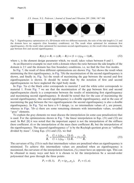
Fig. 7. Eigenfrequency optimization of a 2D domain with two different materials, the ratio of the side length is 2/1 and
the domain have no supports (free boundary conditions). (a) The result when optimized for minimum first
eigenfrequency, (b) the result when optimized for maximum second eigenfrequency, (c) the result when maximizing the
gap between first and second eigenfrequency.
BeðteÞ ¼B1 þ teðB2 B1Þ ¼ð1 þ teðm B 1ÞÞB1, (32)
where te is the element design parameter which, we recall, takes values between 0 and 1.
As an illustrative example we start with a domain where the ratio between the side lengths of the
domain is 2/1 and the domain has free boundary conditions, i.e, we find the free–free modes.
In Fig. 7, the result of three different optimizations are shown: Fig. 7(a) shows the result when
minimizing the first eigenfrequency, in Fig. 7(b) the maximization of the second eigenfrequency is
shown, and finally in, Fig. 7(c) the result of maximizing the gap between the second and first
eigenfrequencies is shown. It should be noted that by the notation of first and second
eigenfrequencies we have neglected the rigid body mode.
In Figs. 7(a–c) the black color corresponds to material 2 and the white color corresponds to
material 1. From Fig. 7 we see that the maximization of the gap between first and second
eigenfrequencies clearly is a compromise between the results of minimizing first eigenfrequency
and maximizing second eigenfrequency. It should be noted that for the case of maximizing the
second eigenfrequency, this second eigenfrequency is a double eigenfrequency, and in the case of
maximizing the gap between the two eigenfrequencies the second eigenfrequency is also a double
eigenfrequency. In Fig. 7(a) we have a 0–1 design, i.e. no intermediate values of te are present,
whereas in Figs. 7(b–c) there are some remaining elements with intermediate values, so-called
‘‘gray’’ elements.
To explain the gray elements we must discuss the interpolation (in some case penalization) that
is used. For the optimizations shown in Fig. 7 the linear interpolation in Eqs. (31) and (32) are
used. In Ref. [8] it was noted that the important aspect is not the interpolation of the stiffness
(here coefficient A) or the interpolation of the mass (here coefficient B), but the interpolation of
the eigenfrequency. The squared eigenfrequency o2 is by the Rayleigh quotient given as ‘‘stiffness
divided by mass’’. Using Eqs. (31) and (32), we find
Ae
¼
Be
ð1 þ teðmA 1ÞÞ A1
¼ f ðteÞ
ð1 þ teðmB 1ÞÞ B1
A1
. (33)
B1
The curvature of Eq. (33) is such that intermediate values are penalized when an eigenfrequency is
minimized. To achieve this intermediate values are penalized when an eigenfrequency is
maximized, the curvature of the interpolation function, f ðteÞ must have an opposite sign. This can
be obtained in many ways and here it is chosen to let the interpolation be a second-order
polynomial that goes through the three points
P1 ¼ð0; 1Þ; P2 ¼ðp2x; p2yÞ; P3 ¼ð1; aÞ.