WAVES AND VIBRATIONS IN INHOMOGENEOUS STRUCTURES ...

Inverse design of phononic crystals by tobology optimization 897
While the above PDEs may be solved analytically for
uniform and homogeneous beams, numerical methods like
the FE Method must be resorted to when considering periodic
in-homogeneous structures as will be the case here.
Let a base cell of length d be divided into N finite elements.
For longitudinal wave motion, the N þ 1 degrees
of freedom (d.o.f) are the nodal longitudinal displacements,
while for bending waves the 2(N þ 1) d.o.f. are the
nodal transverse displacements and the rotation of the
cross-section. For each of the two wave type problems, the
global stiffness matrix K and mass matrix M for the base
cell are assembled in the usual manner from the corresponding
element matrices. For longitudinal waves the element
matrices are 2 2 matrices using first order polynomials
as shape function for u [15]. For bending waves, the
element matrices are 4 4 matrices using third and second
order polynomials as shape functions for w and q
respectively [14]. According to Bloch theory [16], the periodic
boundary condition at the ends of the base cell becomes
for longitudinal waves
uN ¼ u1 e ikB
where k B ¼ kd is the Bloch parameter and k the wave
number. Due to reasons of periodicity, 0 k B p. Similarly
for bending waves, the periodic boundary conditions
become
wN ¼ w1 e ikB
;
qN ¼ q1 e ikB
:
These boundary conditions must be incorporated into the
corresponding stiffness matrices.
Assuming time harmonic motion with circular frequency
w the two eigenvalue problems become
Kiðk B Þ ui ¼ liMiui ; li ¼ w 2 i ; i ¼ L; B ð10Þ
where ui contains the nodal values of the variables, L ¼
longitudinal waves and B ¼ bending waves. The dependence
on k B is shown explicitly.
The stiffness and mass matrices K and M depend in
general on the cross-sectional geometry, length of base cell
and material parameters. Here we choose a fixed circular
cross-section of radius r ¼ 0:5 cm, such that we end up
with only the longitudinally varying material properties
and the cell length as design variables. As discussed in the
previous section, the goal is to find the distribution of two
a priori chosen materials in the base cell, that results in the
largest band gaps as calculated by (10). We choose a continuous
design variable 0 z e 1, z e ¼ 1; ...; N for each
element, that interpolates between the two chosen materials.
In our model (10), there are three material parameters
E, q and n introduced above. We thus have the following
three material interpolation functions on the form (2)
EðzeÞ¼ ð1 zeÞ E1 þ zeE2 ;
qðzeÞ¼ ð1 zeÞ q1 þ zeq2 ;
nðzeÞ¼ ð1 zeÞ n1 þ zen2 :
The subscript i ¼ 1; 2 denotes one of the two materials.
Finally, we also let the base cell length d be a design
parameter, such that the cell length can be optimized.
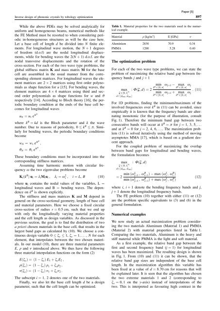
Table 1. Material properties for the two materials used in the numerical
example.
Material q [kg/m 3 ] E [GPa] n
Aluminium 2830 70.9 0.34
PMMA 1200 5.28 0.40
The optimization problem
For each of the two wave type problems, we can state the
problem of maximizing the relative band gap between frequency
bands j and j þ 1
max
z 2½0; 1Š N
: Fðz; dÞ ¼2
d 2½dmin; dmaxŠ
min
k B 2½0; pŠ wjþ1
max
k B 2½0; pŠ wj
min
kB 2½0; pŠ wjþ1 þ max
kB 2½0; pŠ wj
: ð11Þ
For 1D problems, finding the minimum/maximum of the
involved frequencies over k B in (11) can be avoided, since
empirically it is known that the frequency bands are alternating
monotonic (for the purpose of illustration, consult
Fig. 1). Therefore the minimum band gap between two
consecutive bands will occur at k B ¼ p for j ¼ 1; 3; 5; ...
and at k B ¼ 0 for j ¼ 2; 4; 6; .... The maximization problem
(11) is solved iteratively using the method of moving
asymptotes MMA [17], which is based on a gradient descent
approach.
For the coupled problem of maximizing the overlap
between band gaps for longitudinal and bending waves,
the formulation becomes
max
z 2½0; 1Š N
: Fðz; dÞ
d 2½dmin; dmaxŠ
¼ 2 min ðwL jþ1 ; wB iþ1 Þ max ðwL j ; wB i Þ
min ðw L jþ1 ; wB iþ1 Þþmax ðwL j ; wB i Þ
ð12Þ
where i, i þ 1 denote the bending frequency bands and j,
j þ 1 denote the longitudinal frequency bands.
The FE problem (10) together with either (11) or (12)
are the problem specific equivalents to (3) and (6) in the
general formulation.
Numerical examples
We now study an actual maximization problem considering
the two materials Aluminum (Material 1) and PMMA
(Material 2) with material properties listed in Table 1.
Comparing the two materials, Aluminum is the heavy and
stiff material while PMMA is the light and soft material.
As a first example, the relative band gap between the
first and second frequency band (j ¼ 1) for longitudinal
waves has been maximized. The resulting design is shown
in Fig. 1. From (10) and (11) it can be shown, that the
relative band gap sizes are independent of the base cell
length. In the maximization algorithm this variable has
been fixed at a value of d ¼ 8:70 cm for reasons that will
be explained later. It is seen that the algorithm has chosen
the two extreme materials 1 and 2 (corresponding to
z e ¼ 0; 1 on the y-axis) instead of interpolations of the
two. This is interpreted as favouring high contrast in the