

WAVES AND VIBRATIONS IN INHOMOGENEOUS STRUCTURES ...
WAVES AND VIBRATIONS IN INHOMOGENEOUS STRUCTURES ...
WAVES AND VIBRATIONS IN INHOMOGENEOUS STRUCTURES ...

You also want an ePaper? Increase the reach of your titles
YUMPU automatically turns print PDFs into web optimized ePapers that Google loves.
1190 B.S. Lazarov, J.S. Jensen / International Journal of Non-Linear Mechanics 42 (2007) 1186 –1193<br />
ω/κ<br />
1.7<br />
1.6<br />
1.5<br />
1.4<br />
1.3<br />
1.3<br />
1.2<br />
1.2<br />
0<br />
0.01<br />
1.1<br />
1.1<br />
0.05<br />
0.1<br />
1<br />
1<br />
0.2<br />
0.5<br />
0.9<br />
0.9<br />
0 0.2 0.4 0.6 0.8 1 1.2 1.4 1.6 1.8 0 0.2 0.4 0.6 0.8 1 1.2 1.4 1.6 1.8 2<br />
ω/κ<br />
Re(μ u ) Im(μ u )<br />
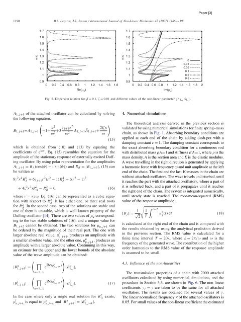
Fig. 5. Dispersion relation for = 0.1, = 0.01 and different values of the non-linear parameter A1,j Ā1,j .<br />
A1,j+1 of the attached oscillator can be calculated by solving<br />
the following equation:<br />
<br />
B1,j+1=A1,j+1 −1+ 2<br />
2 +3 j+12 <br />
2i<br />
A1,j+1Ā1,j+1+ 2 <br />
(15)<br />
which is obtained from (10) and (13) by equating the<br />
coefficients of e it . Eq. (15) resembles the equation for the<br />
amplitude of the stationary response of externally excited Duffing<br />
oscillator. By using polar representation for the amplitudes<br />
A1,j+1 = RA(cos() + i sin()) and RB =|B1,j+1|, (15) can<br />
be written as<br />
9 2 r 4 R 6 A + 6 j+1r 2 (r 2 − 1)R 4 A + ((r2 − 1) 2<br />
+ 4 2 r 2 )R 2 A − R2 B = 0, (16)<br />
where r = /. Eq. (16) can be represented as a cubic equation<br />
with respect to R2 A . It has either one, or three real roots<br />
for R2 A . In the second case, two of the solutions are stable and<br />
one of them is unstable, which is well known property of the<br />
Duffing oscillator [14]. There are two values of u corresponding<br />
to the two stable solutions of (16), and a unique value for<br />
B1,j+2 cannot be obtained. The two solutions for u,j+1 can<br />
be ordered by the magnitude of their real part. The one with<br />
larger absolute real value, l u,j+1 , produces an amplitude with<br />
a smaller absolute value, and the other one, u u,j+1 , produces an<br />
amplitude with a larger absolute value. Continuing in this way,<br />
an estimate for the upper and the lower bounds of the absolute<br />
value of the wave amplitude can be obtained:<br />
|B u 1,j+k |=<br />
<br />
<br />
e Re(u u,j+n )<br />
<br />
|B u 1,j |,<br />
|B l 1,j+k |=<br />
n=1...k<br />
<br />
n=1...k<br />
e Re(l u,j+n )<br />
<br />
|B l 1,j |. (17)<br />
In the case where only a single real solution for R 2 A exists,<br />
l u,j+k is equal to u u,j+k and |Bu 1,j+k |=|Bl 1,j+k |.<br />
1.7<br />
1.6<br />
1.5<br />
1.4<br />
4. Numerical simulations<br />
The theoretical analysis derived in the previous section is<br />
validated by using numerical simulations for finite spring–mass<br />
chain, as shown in Fig. 1. Absorbing boundary conditions are<br />
applied at each end of the chain by adding dash-pot with a<br />
damping constant c = 1. The damping constant corresponds to<br />
the exact absorbing boundary condition for a continuous rod<br />
with distributed mass A=1 and stiffness EA=1, where is the<br />
mass density, A is the section area and E is the elastic modulus.<br />
A wave travelling in the right direction is generated by applying<br />
a harmonic force with frequency and unit amplitude at the left<br />
end of the chain. The first and the last 10 masses in the chain are<br />
without attached oscillators. The wave travels undisturbed, until<br />
it reaches the part with the attached oscillators, where a part of<br />
it is reflected back, and a part of it propagates until it reaches<br />
the right end of the chain. The system is integrated numerically,<br />
until steady state is reached. The root-mean-squared (RMS)<br />
value of the response amplitude<br />
[Bj ]= 1<br />
<br />
<br />
1 t+T<br />
√ u<br />
2 T t<br />
2 j (t) dt (18)<br />
is calculated at the right end of the chain and is compared with<br />
the results obtained by using the analytical prediction derived<br />
in the previous section. The RMS value is calculated for a<br />
finite time interval T = 20, where = 2/ and is the<br />
frequency of the generated wave. The contribution of the higher<br />
order harmonics to the RMS value of the response amplitude<br />
is assumed to be small.<br />
4.1. Influence of the non-linearities<br />
The transmission properties of a chain with 2000 attached<br />
oscillators calculated by using numerical simulations, and the<br />
procedure in Section 3.3, are shown in Fig. 6. The non-linear<br />
coefficients j = are taken to be the same for all attached<br />
oscillators. The results are obtained for several values of .<br />
The linear normalised frequency of the attached oscillators is<br />
0.05. For small values of the non-linear coefficient the estimated


