WAVES AND VIBRATIONS IN INHOMOGENEOUS STRUCTURES ...

ω/κ
ω/κ
1.5
1.4
1.3
1.2
1.1
1
0.9
0.8
0.7
B.S. Lazarov, J.S. Jensen / International Journal of Non-Linear Mechanics 42 (2007) 1186–1193 1189
ω/κ
0.6
0.6
0 0.1 0.2 0.3 0.4 0.5 0.6 0.7 0.8 0.9 0.1 0.2 0.3 0.4 0.5 0.6 0.7 0.8 0.9 1 1.1
1.5
1.4
1.3
1.2
1.1
1
0.9
0.8
0.7
0.6
1.5
1.4
1.3
1.2
1.1
1
Re(μ u ) Im(μ u )
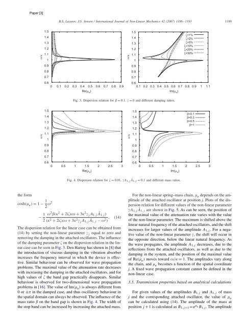
Fig. 3. Dispersion relation for = 0.1, = 0 and different damping ratios.
0 0.5 1 1.5 2 2.5 3
ω/κ
0.9
0.8
0.7
1.5
1.4
1.3
1.2
1.1
1
Re(μ u ) Im(μ u )
0.9
0.8
0.7
0.6
ζ=1%
ζ=2%
ζ=5%
ζ=10%
ζ=20%
ζ=30%
β=0.1
β=0.3
β=0.5
β=1
0 0.5 1 1.5 2 2.5
Fig. 4. Dispersion relation for = 0.01, A1,j Ā1,j = 0.1 and different mass ratios.
the form
cosh(u) = 1 − 1
2 2
− 1
2
2(2 + 2i + 32j A1,j Ā1,j )
(2 + 2i + 32j A1,j Ā1,j − 2 . (14)
)
The dispersion relation for the linear case can be obtained from
(14) by setting the non-linear parameter j equal to zero and
removing the damping in the attached oscillators. The influence
of the damping parameter on the dispersion relation in the linear
case can be seen in Fig. 3. Den Hartog has shown in [8] that
the introduction of viscous damping in the vibration absorber
increases the frequency interval in which the device is effective.
Similar behaviour can be observed for wave propagation
problems. The maximal value of the attenuation rate decreases
with increasing the damping in the attached oscillators, and for
high values of the band gap practically disappears. Similar
behaviour is observed for two-dimensional wave propagation
problems in [16]. The value of Im(u) is always different from
0or± in the damped case, and thus oscillatory behaviour in
the spatial domain can always be observed. The influence of the
mass ratio on the band gap is shown in Fig. 4. The width of
the stop band can be increased by increasing the attached mass.
For the non-linear spring–mass chain, u depends on the amplitude
of the attached oscillator at position j. Plots of the dispersion
relation for different values of the non-linear parameter
A1,j Ā1,j are shown in Fig. 5. As can be seen, the position of
the maximal value of the attenuation rate varies with the value
of the non-linear parameter. The maximum is shifted above the
linear natural frequency of the attached oscillators, and the shift
increases for larger values of the amplitude A1,j .Foranegative
value of the non-linear parameter , the shift will occur in
the opposite direction, below the linear natural frequency. As
the wave propagates, the amplitude A1,j decreases, due to the
reflections from the attached oscillators, as well as due to the
damping in the system, and the position of the maximal value
of Re( u) moves toward / = 1. The amplitudes vary along
the chain, and u becomes a function of the spatial coordinate
j. A fixed wave propagation constant cannot be defined in the
non-linear case.
3.3. Transmission properties based on analytical calculations
For given values of the amplitudes B1,j and A1,j of mass
j and the corresponding attached oscillator, the value of u
can be calculated using (14). The amplitude of the mass at
position j +1 is calculated as B1,j+1 =e uB1,j . The amplitude
3