WAVES AND VIBRATIONS IN INHOMOGENEOUS STRUCTURES ...

1188 B.S. Lazarov, J.S. Jensen / International Journal of Non-Linear Mechanics 42 (2007) 1186 –1193
ω
2
1.8
1.6
1.4
1.2
1
0.8
0.6
0.4
0.2
0
0 2 4 6
The time response of qj (t) is assumed to be periodic in the
form of complex Fourier series
qj (t) =
(k−1)/2 Ak,je ikt + (k−1)/2 Āk,je −ikt ,
k
k = 1, 3,..., (9)
where is a dimensionless bookkeeping parameter showing the
order of the amplitude of the motion. By substituting (9) into
(5) and integrating twice with respect to time, the following
expression for the time response of mass j can be obtained:
uj (t) = A1,j −1 + 2
2 + 3 j 2 2 A1,j Ā1,j + 2i
e
it
+ −A3,j + 2 i
3 A3,j + 1
9
2
2 A3,j + 1 j
9
2
2 A3
1,j
× e i3t + c.c. + O( 2 ). (10)
The expression in the above equation is obtained by truncating
the time series and preserving only the first two terms. By
substituting (10) and (9) into (4) and equating to zero the coefficients
in front of e ikt , a system of algebraic equations for
the amplitudes Ak,j can be obtained
2
2 − 1 +
2 2 − 1 2 + 2i
(2 − 1 2
) A1,j
2
+ 3j 2 (2 − 1 2 )A 2 1,j Ā1,j
+ 1 − 2
− 2i
2
− 3 j+1
(A1,j+1 + A1,j−1)
2 2 A21,j+1Ā1,j+1
− 3j−1 2
2 A21,j−1Ā1,j−1 = 0,
∞
ω
Re(μ u ) Im(μ u )
2
1.8
1.6
1.4
1.2
1
0.8
0.6
0.4
0.2
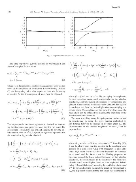
Fig. 2. Dispersion relation for = 1.0 and = 0.1.
(11)
2
0
0 0.5 1 1.5 2 2.5 3 3.5
2
2 3
− 1 + 2 3 − 1 2 + 2i
(2 − 1 2 3 )
3
+ 2 2
2 − 1 3
2
j A 3 1,j +
1 − 2
2 − 2i
3
3
× (A3,j+1 + A3,j−1)
− j+1
2
2 3
A 3 1,j+1 − j−1
2 2 A
3
3 1,j−1
A3,j
= 0, (12)
where 1 = + 1 and 3 = 3. By specifying the amplitudes
for two neighbour masses and, respectively, for the attached
oscillators, a solvable system of equations for the response amplitudes
of the attached oscillators can be obtained. The system
is non-linear and there can be multiple solutions satisfying it in
certain cases. The amplitude of the wave travelling along the
main chain can be obtained by inserting the amplitude of the
attached oscillators into (10).
The wave travelling along the spring–mass chain can also
be investigated by using the wave number multiplied by
the distance between the masses in the main chain u. The
displacements of the masses neighbour to mass j can be
expressed as
uj±1 =
k
Bk,je ± u k e ikt + c.c., (13)
where Bk,j are the coefficients in front of e ikt from Eq. (10).
It can be clearly seen that the solution in the non-linear case
consists of a zero order wave with frequency and additional
high order waves. As the non-linearities are assumed
to be small and the focus is on the filtering properties of
the chain around the linear natural frequency of the attached
oscillators, the contributions to the solution of the harmonics
of order equal to and higher than k = 3 are neglected. Substituting
(13) and (9) into (4), equating the coefficients in front of
e it to zero and solving the resulting equation with respect to
u, the dispersion relation for the non-linear case is obtained in